Features RSS

star cluster IC 348 as seen by JWST

Last year, a researcher claimed the first detection of an amino acid, tryptophan, in an interstellar cloud. New research that leverages laboratory experiments and data from JWST refutes this finding, suggesting that the hunt for the first amino acid in the interstellar medium isn’t over yet.

A Hunt for Amino Acids

Researchers have long sought evidence for amino acids, the building blocks of all life on Earth, in the dusty clouds of the interstellar medium. Several amino acids have turned up in meteorites and the gaseous envelopes of protostars, but claimed detections of these critical molecules in cold, star-forming clouds have been refuted. Now, another potential detection awaits confirmation.

diagram of a tryptophan molecule

The structure of a tryptophan molecule. [Dhariwal et al. 2024]

The amino acid in question is tryptophan, which is perhaps best known for being unfairly blamed for post-Thanksgiving sleepiness due to its presence in turkey meat. Research published in 2023 found evidence for tryptophan in the gas suffusing the star cluster IC 348, based on a comparison of an infrared spectrum from the Spitzer Space Telescope to a laboratory spectrum of the molecule. How does this finding hold up to further tests?

comparison of results from new and previous laboratory spectra of tryptophan

Comparison of the Spitzer spectrum used in the claimed detection of tryptophan (orange) to the new laboratory spectrum (blue) and the previously used laboratory spectrum (red). The panels at the bottom show individual spectral features. Click to enlarge. [Dhariwal et al. 2024]

A Three-Pronged Investigation

Aditya Dhariwal (University of British Columbia) and collaborators used several methods to evaluate the claimed detection, beginning with a laboratory spectrum of the molecule. It’s no easy task to simulate the conditions of the interstellar medium in a lab: the density of interstellar gas can be far lower than the best lab vacuum, and temperatures in cold clouds hover just above absolute zero. This makes it challenging to generate spectra that match what would be seen from molecules in interstellar space.

The previous study used a lab spectrum of tryptophan in the form of a solid pellet. Dhariwal’s team pointed out that unlike in the interstellar medium, tryptophan in a solid state likely takes the form of a zwitterion: a molecule that has no electric charge overall but is composed of parts that carry electric charge.

The team used a new method to prepare a sample of tryptophan in non-zwitterionic form and compared the collected infrared spectrum to the Spitzer observations. Crucially, the spectral lines seen by Spitzer and assigned to tryptophan have no matches in the new spectrum.

Paths Forward

JWST spectrum of IC 348

Spectrum of IC 348 from JWST (top) and individual spectral lines from that spectrum (bottom). The blue dotted lines mark the locations of the reported tryptophan lines. Click to enlarge. [Dhariwal et al. 2024]

Next, the team analyzed new infrared spectra of IC 348 from JWST. The JWST spectra clearly contained spectral lines from hydrogen and other elements in the cloud, but none of the lines attributed to tryptophan were present.

Finally, Dhariwal’s team revisited the Spitzer observations used in the previous analysis. Their examination of the spectrum led them to suspect that the purported emission lines of tryptophan were instrumental artifacts rather than true spectral lines.

This study demonstrates the fascinating back and forth of science at work. Although the latest investigation finds no compelling evidence for tryptophan in the interstellar medium, the authors identified paths forward. Laboratory spectra of tryptophan gas at radio wavelengths allow for searches of the sky at longer wavelengths, and though challenging to collect, spectra of tryptophan gas at infrared wavelengths could open yet another window. The search goes on!

Citation

“On the Origin of Infrared Bands Attributed to Tryptophan in Spitzer Observations of IC 348,” Aditya Dhariwal et al 2024 ApJL 968 L9. doi:10.3847/2041-8213/ad4d9a

photograph of runaway star Zeta Ophiuchi

A substantial number of O and B stars say goodbye to their birth clusters and spend their lives zooming through space alone. New research uses the most recent Gaia data to investigate the properties of these runaway stars.

Massive Stars Far from Home

The Trapezium cluster

OB stars are typically born in clusters, like the Trapezium Cluster at the heart of the Orion Nebula, shown here. [ESO/IDA/Danish 1.5 m/R.Gendler, J.-E. Ovaldsen, and A. Hornstrup; CC BY 4.0]

The majority of the most massive stars in our galaxy — those with spectral types O and B, also called OB stars — live and die within their natal star clusters, never traveling far from where they were born during their brief, luminous lives. But roughly 20–30% of OB stars lead significantly more adventurous lives. So-called runaway stars careen through space on a solo adventure or with a single companion, traveling light-years from their birthplaces.

Stars can be ejected from their birth clusters by dynamical interactions or supernova explosions. Dynamical ejection happens when stars in a crowded cluster pass too close to one another, slingshotting one or more stars into space. A star that explodes as a supernova can expel its close binary companion from the cluster. In rare cases, the exploding star and its companion can escape the cluster together. It’s not yet known which process creates more runaway stars or how the two populations of runaways differ.

Map of the Small Magellanic Cloud with stellar proper motion vectors for potential runaway stars

Vectors showing the motion across the sky of the stars in the authors’ sample. Eclipsing binaries (EB) and double-lined spectroscopic binaries (SB2) were ejected dynamically. High-mass X-ray binaries (HMXB) have experienced a supernova. Click to enlarge. [Phillips et al. 2024]

A Search for Runaway Stars

Diving into this question, a team led by Grant Phillips (University of Michigan) investigated more than 300 potential runaways in a nearby dwarf galaxy, the Small Magellanic Cloud. The stars in their sample were chosen for being at least 90 light-years from other OB stars (with the exception of stars in binary systems, which may have escaped their home cluster together).

The binary systems in the sample immediately gave away how they were launched into space: binary systems that don’t contain a neutron star or a black hole can’t have experienced a supernova — those binaries must have been kicked out of their clusters through dynamical interactions. Binary systems that do contain a neutron star or a black hole must have experienced a supernova. As for solo runaway stars, the team’s earlier research suggested that typical OB stars tend to be expelled through dynamical interactions, while stars with emission lines in their spectra due to rapid rotation — OBe stars — tend to be ejected by supernovae.

Population Comparison

Mass and velocity distributions for stars ejected dynamically and via supernovae

Mass and velocity distributions for stars ejected dynamically (left) and via supernovae (right). Click to enlarge. [Phillips et al. 2024]

Using the third release of Gaia spacecraft data, Phillips’s team calculated the velocities of the stars in their sample. They found that the velocities of the single OBe stars overlapped well with those of the post-supernova binary systems, although the OBe stars’ velocities extended to higher values. While this could be an effect of small-number statistics, it could also be due to some stars reaching high velocities through a two-step process: first, dynamical ejection as a member of a binary system; then, an extra velocity kick when the binary companion goes supernova.

The velocities of typical OB stars are similar to the velocities of binary systems ejected dynamically, supporting the hypothesis that these stars are also ejected this way. Intriguingly, the velocity distribution for typical OB stars may have two peaks. The authors speculate that the peaks could point to two groups of dynamical interactions: stars ejected by just a single other star versus stars ejected by a binary system.

Underpinning these findings is the rich, precise dataset from Gaia, which allowed the team to identify systematic offsets from their previous work based on earlier data releases from the spacecraft. Hopefully, future data releases can give even more clues to the origins of these runaway stars!

Citation

“Runaway OB Stars in the Small Magellanic Cloud. III. Updated Kinematics and Insights into Dynamical versus Supernova Ejections,” Grant D. Phillips et al 2024 ApJ 966 243. doi:10.3847/1538-4357/ad3909

Illustration of ejecta from the collision of two neutron stars

Roughly thirteen billion years ago, the periodic table was easy to memorize: hydrogen, helium, and lithium were the only chemical constituents of the infant universe. Today, things are a little more complicated. Through billions of years of stellar alchemy, the universe is now awash with an abundance of metals — what astronomers call elements heavier than helium. Some of these metals are forged in the cores of stars, while others require explosive events to form. In today’s post, we’ll take a look at three research articles that examine the creation of heavy elements in exotic environments across the universe.

Making Metals in Supernovae

Core-collapse supernovae are one of the sites of element formation, which is also called nucleosynthesis. Core-collapse supernovae are triggered by the collapse of a massive star as the star exhausts its ability to hold off the inward pressure of gravity with the outward pressure of radiation generated by nuclear reactions in its core. When the star’s core collapses, its outer layers recoil from the condensed core and explode into space.

The hot, dense ejecta of a supernova explosion may be a good place for elements to be created through r-process nucleosynthesis. In this process, multiple free-wheeling neutrons pack onto nearby atoms, creating heavier isotopes and elements fast enough that unstable isotopes don’t have the chance to decay. (The counterpart to the rapid r-process is the slow s-process, in which a trickle of neutrons builds elements and isotopes more gradually. The s-process tends to take place in stellar interiors, without the need for a cataclysmic explosion.) It’s not yet clear how much element creation via the r-process happens in core-collapse supernovae or how this quantity depends on the mass of the star or other factors.

plots of modeled supernova light curves

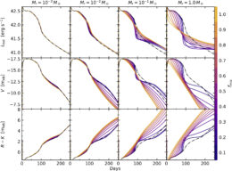
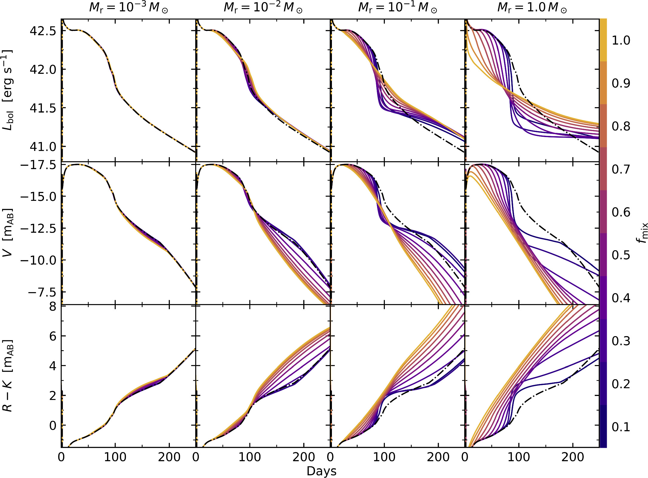
Modeled supernova light curves showing the impact of increasing the amount of r-process material (Mr) and the degree of mixing (fmix). Click to enlarge. [Patel et al. 2024]

Anirudh Patel (Columbia University) and collaborators used simulations to understand how r-process nucleosynthesis might leave its mark on the light curves of core-collapse supernovae. Patel’s team produced one set of models in which no r-process reactions take place and another in which r-process elements are produced deep within the explosion and then mixed throughout the ejected material. The team varied the amount of r-process material and how thoroughly it’s mixed with other material.

Patel and coauthors found that if the amount of r-process material is small — less than a hundredth of the mass of the Sun — the light curve looks scarcely different than if there is no r-process material at all. For larger amounts of r-process material and greater degrees of mixing, the “plateau” phase of the light curve shortens and dims, and the supernova appears redder than it otherwise would. The team’s research suggests that r-process-enriched supernovae should be distinguishable from regular supernovae but may be confused with certain types of rare supernovae.

The Influence of Magnetic Fields

Many core-collapse supernovae leave behind a neutron star: an extraordinarily dense sphere of neutrons about 10 kilometers in radius and about the mass of the Sun. When two neutron stars collide, the merger creates ideal conditions for element formation through the r-process. In a recent article, Kelsey Lund (North Carolina State University and Los Alamos National Laboratory) and collaborators examined element creation in the case of a neutron star merger than produces a black hole surrounded by a hot, dense accretion disk.

plots of modeled total ejecta mass, lanthanide mass, and actinide mass as a function of magnetic field strength

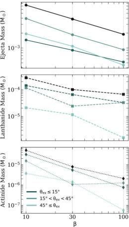
Total ejecta mass, lanthanide mass, and actinide mass as a function of magnetic field strength (lower β corresponds to a stronger magnetic field) and the angle of the outflow. Note the different y-axis scales in the middle and bottom plots. [Adapted from Lund et al. 2024]

The merger of a binary pair of neutron stars can create a bright electromagnetic signal called a kilonova. The kilonova emission is powered by the radioactive decay of r-process elements that are produced when the stars collide. One of the many uncertainties that surround the creation of a kilonova is the impact of the magnetic field. The magnetic field is thought to control how quickly material flows from the accretion disk onto the black hole as well as how rapidly the material flows out from the disk — two factors that influence the production of r-process material.

Lund’s team used general relativistic magnetohydrodynamics simulations to trace the evolution of the disk that forms after the stars merge. The three simulations capture the nucleosynthesis that occurs within about 127 milliseconds of the collision. When the magnetic field is stronger, more mass is ejected by the merger and larger amounts of elements in the lanthanide and actinide groups — the two rows of heavy elements separated from the rest of the periodic table — are produced. The amounts of lanthanide-group and actinide-group elements both increase with increasing magnetic field strength, but the increase is larger for the actinide-group elements.

This last finding could explain a curious feature of some old stars: while many old stars contain about the same amount of lanthanide-group elements, there is a broad range of actinide-group element abundances. This may reflect the different magnetic field conditions in the neutron star mergers where the elements formed, long before the stars themselves were born.

Collapsar Jets and Nucleosynthesis

The final article of today’s post examines a variety of element-making methods in the aftermath of a collapsar: a rapidly spinning, massive star that collapses into a black hole, slinging jets of material into space in the process. Zhenyu He (Beihang University) and collaborators used an extensive network of nuclear reactions to model the fusion, fission, and decay taking place in the collapsar’s jets.

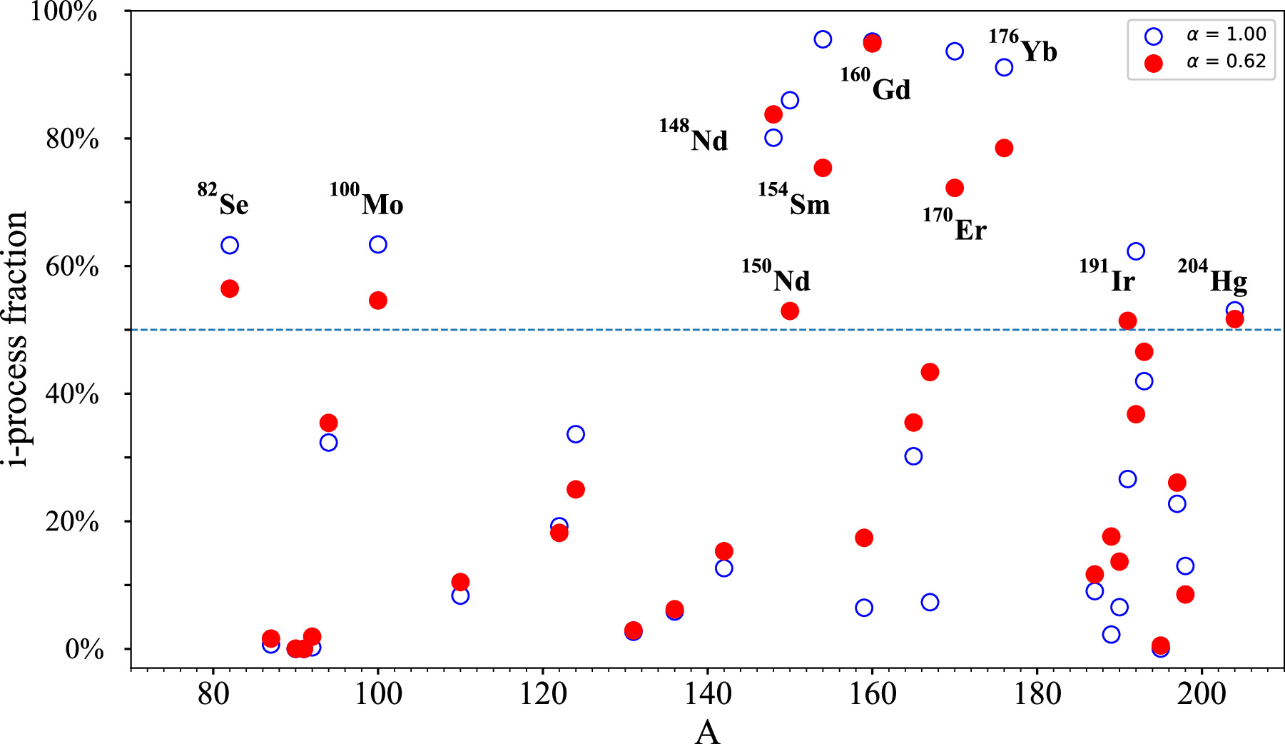
He’s team found that in the immediate aftermath of a collapsar, the r-process is in full swing, packing neutrons onto outflowing atoms and forming elements like gold and platinum. After about five seconds, the outflow has cooled enough that the r-process stalls. This doesn’t mean that nucleosynthesis stops, though: the team found evidence that the slower s-process and the intermediate-speed i-process take over and continue to churn out heavier atomic species for several hours. The later, slower nucleosynthesis is mainly powered by neutrons from the fission of fermium and rutherfordium.

plot of i-process fraction as a function of atomic number

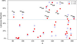
Percentage of element yield (A = atomic mass in atomic mass units) from the i-process. Many elements’ yields are greatly enhanced by the i-process. The two sets of symbols represent results from simulations with different expansion rates. Click to enlarge. [He et al. 2024]

Previous modeling of other r-process sites like supernovae has not revealed this later stage of nucleosynthesis, but this work suggests that the s-process and i-process are important for shaping the chemical makeup of collapsar outflows. In particular, the pattern of elements with even numbers of protons being more abundant than elements with odd numbers of protons might be enhanced by these processes. To learn more, He’s team proposed, researchers will need to study old, metal-poor stars in the distant halo of the Milky Way, which may have formed from gas enriched by collapsars rather than neutron star mergers.

Citation

“The Effects of r-Process Enrichment in Hydrogen-Rich Supernovae,” Anirudh Patel et al 2024 ApJ 966 212. doi:10.3847/1538-4357/ad37fe

“Magnetic Field Strength Effects on Nucleosynthesis from Neutron Star Merger Outflows,” Kelsey A. Lund et al 2024 ApJ 964 111. doi:10.3847/1538-4357/ad25ef

“Possibility of Secondary i– and s-Processes Following r-Process in the Collapsar Jet,” Zhenyu He et al 2024 ApJL 966 L37. doi:10.3847/2041-8213/ad444c

debris disk surrounding Fomalhaut C

JWST has achieved another first: the telescope has spotted light scattered by dust grains in the debris disk surrounding the star Fomalhaut C for the first time. These observations add to our knowledge of the planet formation process around the smallest and most common stars in our galaxy.

A Fleeting Phase

As stars and planets form out of collapsed clouds of gas and dust, nascent planetary systems pass through a short and poorly understood phase. Lasting just 10 million years, the fleeting debris disk stage is marked by collisions between protoplanets that create disks or rings of dust and rubble.

Studying debris disks is key to understanding how planetary systems form. Very few debris disks have been seen around the smallest, coolest, and most common type of star in the Milky Way — M dwarfs —and detailed observations of the few known M-dwarf debris disks have been scarce. Studies are split on whether low-mass stars are less likely to host debris disks or if these disks are simply more challenging to detect. Luckily, JWST is capable of spotting these elusive disks, and recent observations have given researchers a new perspective on a disk surrounding an M dwarf just 25 light-years away.

Disk Detected

photograph of the debris disk surrounding Fomalhaut A

ALMA’s view of the debris disk around Fomalhaut A. [ALMA (ESO/NAOJ/NRAO); M. MacGregor; CC BY 3.0]

Fomalhaut is a triple-star system most famous for the debris disk and highly debated planet candidate around the largest and brightest star in the system, Fomalhaut A. Astronomers previously spotted thermal emission from a debris disk surrounding an M dwarf in the system, Fomalhaut C, in observations by the Atacama Large Millimeter/submillimeter Array (ALMA), but follow-up observations failed to spot the disk in scattered light. Scattered-light observations give researchers valuable information about the size and makeup of dust grains in the disk.

Recently, a team led by Kellen Lawson (NASA’s Goddard Space Flight Center) turned JWST toward Fomalhaut C and eight other nearby M dwarfs to search for planets around these stars. In JWST’s 3.56 and 4.44 micron (1 micron = 10-6 meter) filters, the authors detected a faint disk extending beyond the star. In the shorter-wavelength filter, the outline of the disk matched the location of the debris disk seen previously by ALMA. In the longer-wavelength filter, the disk extended slightly beyond the emission seen by ALMA.

Challenging Observations

Fomalhaut C is the smallest and coolest star for which a disk has been detected in scattered light. The new observations highlight JWST’s ability to track down debris disks around small, cool stars, as well as the inherent difficulty of observing these structures: even under JWST’s watchful gaze, the star’s debris disk is seen only faintly, with background objects and noise interfering with the telescope’s view.

several views of Fomalhaut C's debris disk

Fomalhaut C’s disk as seen in two different filters and with several different methods of removing diffracted starlight. Click to enlarge. [Lawson et al. 2024]

The difficult observing conditions complicated analysis of the disk’s properties — a challenging background-light subtraction might be responsible for the unaccountably red color of the disk — but the team was still able to search for planets. Lawson’s team ruled out the presence of a planet with a mass higher than Saturn’s mass orbiting within a distance of 10 au or a planet with a mass higher than Jupiter’s orbiting the star within 5 au.

Follow-up observations of Fomalhaut C may refine our understanding of its debris disk, and future observations with JWST are sure to add to the small but critical sample of debris disks surrounding the smallest stars.

Citation

“JWST/NIRCam Detection of the Fomalhaut C Debris Disk in Scattered Light,” Kellen Lawson et al 2024 ApJL 967 L8. doi:10.3847/2041-8213/ad4496

Illustration showing a distant galaxy emitting a pulse of light that passes through the halo of an intervening galaxy and arrives at the Milky Way.

What is the source of radio transients? Astronomers still aren’t sure, but that’s not stopping them from modeling their observations of these mysterious flashes.

The Challenge of Modeling a Mystery

Imagine a radio astronomer in the first moments following an alert that their telescope just recorded something strange in the sky. Their computer informs them that for barely a millisecond, it spotted a mighty flash of radio waves (aptly called a fast radio burst), but before any humans knew something was happening, the flash had already faded. What was that?

In some fields of astronomy, the next steps would be obvious. The scientist would need to write a model that simulates the physics of some known system, then fiddle with the input parameters of that model until its outputs resemble their data. This radio astronomer is not so lucky, though. That’s because although there are many good ideas and many theorists actively working on it, scientists still do not know the source of fast radio bursts.

So, what is the radio astronomer to do? How can you fit a model and learn anything about what you just saw when you don’t know what caused it? That’s where the authors of a recent publication led by Emmanuel Fonseca, West Virginia University, come in.

A New Tool

Observed data of a fast radio burst (left), the best-fitting fitburst model (center), and the residuals to the fit (right). Click to enlarge. [Fonseca et al. 2024]

Fonseca and collaborators created a flexible model that is able to reproduce a wide range of different pulse shapes and sizes, then coded it all up as an open-source Python package called fitburst. Some of their input parameters, like the dispersion measure, correspond to physical quantities, and they include every bit of realistic physics that they can. Other input parameters, however, are just heuristics. Fitting all of the parameters in their model won’t tell you why certain frequencies remained dim while others flared, but it will tell you the relationship between frequency and peak brightness.

That’s a crucial intermediate step towards developing a more complete theory of fast radio bursts, since it allows scientists to classify the population of observed bursts even without a full understanding of their underlying cause. Already astronomers have noted that there seem to be at least a few distinct types of fast radio bursts, and with a tool like fitburst, they can begin to quantify the differences between these populations.

Careful and Complete Implementation

A fit to a different fast radio burst, which arrived at several staggered, frequency-dependent times. Click to enlarge. [Fonseca et al. 2024]

Fonseca and the team also derived analytic expressions for the derivatives of each of their input parameters, which unlocked a powerful family of model-fitting algorithms that rely on this extra information to find the best values. In a series of comparisons with real observations of fast radio bursts, they convincingly demonstrate both that these algorithms can find best-fitting solutions, and also that these solutions closely resemble the observed data.

Excitingly, the researchers also noted that the fitburst model is flexible enough to fit other types of pulses as well. Although designed primarily for fast radio bursts, it can also be used to analyze observations of pulsars and other radio transients. The team encourages all radio astronomers to take fitburst for a spin, and they themselves already list four distinct projects underway. The future of fitburst is bright, much like the mysterious flashes it models.

Citation

“Modeling the Morphology of Fast Radio Bursts and Radio Pulsars with fitburst,” E. Fonseca et al 2024 ApJS 271 49. doi:10.3847/1538-4365/ad27d6

projection of the gamma-ray sky

Where do the highest-energy particles in the universe come from? New research suggests that the sources of ultra-high-energy cosmic rays aren’t necessarily the sources of ultra-high-energy photons as well.

Cosmic Rays Across the Universe

Across the universe, extremely energetic charged particles called cosmic rays zoom through space. These particles are usually protons or the bare nuclei of helium atoms, but they can also be electrons, the nuclei of atoms heavier than helium, or other particles like positrons.

Exactly where these particles are accelerated to nearly the speed of light is an open question. One clue to the origin of the most energetic cosmic rays — ultra-high-energy cosmic rays — is that these particles are not distributed evenly across the sky. Any proposed source of ultra-high-energy cosmic rays, like supernovae, gamma-ray bursts, or other highly energetic cosmic beacons, must be able to explain this distribution.

Distribution of resolved extragalactic gamma-ray sources used in this work

Distribution of resolved extragalactic gamma-ray sources used in this work. The color bar indicates the gamma-ray flux of each source. [Partenheimer et al. 2024]

From Energetic Photons to Energetic Particles

Angelina Partenheimer (University of Wisconsin) and collaborators investigated the possibility that the highest-energy cosmic rays and the highest-energy photons have the same source. To test this hypothesis, the team constructed a sample of resolved gamma-ray sources with energies between 50 megaelectronvolts and 1 teraelectronvolt. They then modeled the distribution of ultra-high-energy cosmic rays that might be emitted by this collection of gamma-ray sources.

They used two scenarios to model the cosmic-ray distribution. In the first scenario, the cosmic-ray flux scales with the gamma-ray flux, meaning that sources that are brighter in gamma rays also produce more cosmic rays. In the second scenario, each gamma-ray source appears equally bright in cosmic rays from our vantage point. While this doesn’t reflect reality — it would imply that more distant gamma-ray sources produce more cosmic rays — this treatment may help correct for the fact that catalogs of gamma-ray sources are increasingly incomplete at larger distances.

projection of the modeled cosmic-ray distribution

The modeled cosmic-ray flux for the scenario in which the sources are uniformly bright. The resulting dipole for this scenario is roughly five times larger than what has been observed. [Partenheimer et al. 2024]

Cosmic-Ray Bright, Gamma-Ray Dim?

In both scenarios, the modeled cosmic-ray distribution is far more uneven than what has been observed. Much of the unevenness comes from the extremely bright gamma-ray source Markarian 421, which helps to produce a dipole in the cosmic-ray distribution 5–10 times larger than what has been observed. This suggests that resolved gamma-ray sources alone cannot be the sources of ultra-high-energy cosmic rays; many more sources are needed to balance out the few extremely luminous objects.

Partenheimer’s team found that roughly 80,000 “missing” sources are needed to match the observed distribution of ultra-high-energy cosmic rays. This is far larger than the known population of resolved gamma-ray sources, which could mean that the producers of the highest-energy cosmic rays are unresolved gamma-ray sources. Alternatively — and perhaps surprisingly — the sources of ultra-high-energy cosmic rays might not produce gamma rays at all!

Citation

“Ultra-High-Energy Cosmic-Ray Sources Can Be Gamma-Ray Dim,” Angelina Partenheimer et al 2024 ApJL 967 L15. doi:10.3847/2041-8213/ad4359

photograph of Uranus

Uranus is thought to possess a core of rock and ice beneath its vast frosty atmosphere. Just how much rock lies at the center of this giant world is unknown, but a newly proposed technique could provide a way to find out.

Core Concerns

photograph of Uranus and its rings from JWST

This JWST Near-Infrared Camera image of Uranus shows the planet’s faint ring system and 9 of its 27 moons. [NASA, ESA, CSA, STScI]

When the Voyager 2 spacecraft whizzed past Uranus in January 1986, it revealed the planet’s dark, delicate rings and its pale cyan atmosphere. Precisely what lies beneath the ice giant’s thick atmosphere is unknown, though researchers expect that the planet’s core is made of rock and ice.

But just how much of the core is made of rock is unknown, and it’s likely to be challenging to measure. Space-based measurements of gravitational pull are are often used to infer a planet’s interior density structure. However, if some of Uranus’s atmospheric gas is mixed into the rock, the mixture will have a density similar to that of ice, making it impossible to differentiate between rock and ice using gravity measurements. How, then, can we tell how much rock is in Uranus’s core?

Noble Gas Method

Francis Nimmo (University of California, Santa Cruz) and collaborators proposed that the amount of rock in Uranus’s core could be calculated by measuring the concentration of argon-40 in its atmosphere. Argon-40, a form of the noble gas argon containing 40 neutrons, is the most common type of argon in Earth’s atmosphere.

Argon can be produced through the radioactive decay of potassium, which clings to silicate-rich materials like the rocks thought to be present in Uranus’s core. As potassium slowly decays to argon with a 1.25-billion-year half-life, the newly produced argon diffuses into the planet’s atmosphere. By measuring the amount of argon in Uranus’s atmosphere, Nimmo’s team suggests, researchers can infer the amount of potassium — and rock, by extension — in the planet’s core.

plot of calculated argon-40 concentration

Concentration of argon-40 as a function of the core rock mass in units of Earth masses, ME, and the transport factor, f. [Nimmo et al. 2024]

A Complex Measurement

Nimmo and coauthors find that if the transport of argon from Uranus’s core to its atmosphere is efficient, an atmospheric probe could easily measure the concentration of argon-40. But because there appears to be a trade-off between the mass of the rock core and how efficiently it propels argon-40 into the atmosphere, a spacecraft would need to measure the total mass of the core through gravity measurements or seismology to get a final estimate of how much rock is in the core.

There are other possible complications: some argon in Uranus’s atmosphere was likely already present when the planet was swirled together from the nebula that birthed the Sun and the planets. To disentangle the argon produced in the core from the argon present since the planet’s birth, a visiting spacecraft would need to measure the ratio of argon-40 to argon-36, a form of the element that is produced in supernovae. This ratio would then need to be compared to the primordial ratio of the two forms of argon, which is not known precisely.

The opportunity to test the authors’ theory may lie ahead: a Uranian orbiter and probe was the top priority in the 2023–2032 Planetary Science and Astrobiology Decadal Survey. With two decades or more until the possible arrival of such a spacecraft, scientists have time to contemplate how to measure the makeup of Uranus’s core.

Citation

“Probing the Rock Mass Fraction and Transport Efficiency Inside Uranus Using 40Ar Measurements,” Francis Nimmo et al 2024 Planet. Sci. J. 5 109. doi:10.3847/PSJ/ad3b93

illustration of a white dwarf collecting gas from its stellar companion

With T Coronae Borealis expected to have an outburst any day now, recurrent novae are in the news. Recently, researchers reported their investigation of a recurrent nova that brightens every year.

Recurring Stellar Characters

light curves from M31N 2008-12a's eruptions from 2013 to 2022

Vertically offset light curves from M31N 2008-12a’s 2013–2022 eruptions. [Basu et al. 2024]

Recurrent novae are periodic outbursts that happen when a white dwarf — the exposed core of an evolved star with a mass of about 8 solar masses or less — snags some gas from a puffy red giant companion. Heated by the blisteringly hot surface of the white dwarf, this accreted gas ignites in a flash of nuclear fusion. This process can recur for millions of years, creating with each outburst a “guest” star that fades until the next eruption.

Known recurrent novae have outbursts anywhere from every year to every 98 years. The nova with the most recorded appearances is M31N 2008-12a, which hails from our galactic neighbor, Andromeda. Researchers have witnessed the star brighten 15 times since its discovery in 2008, and a dive into the archives dredged up three previous eruptions in 1992, 1993, and 2001. What can this collection of eruptions tell us about M31N 2008-12a’s past, present, and future?

Light curve showing the overall behavior as well as the "cusp" feature

Light curve in the i’ band, showing the overall behavior as well as the “cusp” feature. Click to enlarge. [Adapted from Basu et al. 2024]

Characterizing Outbursts

Judhajeet Basu (Indian Institute of Astrophysics and Pondicherry University) and collaborators examined optical, ultraviolet, and X-ray data to examine the behavior of M31N 2008-12a during its annual outbursts from 2017 to 2022. Their investigation showed that each outburst was roughly the same — rising rapidly to its peak in about a day, then declining sharply for 2–4 days before fading more gradually.

In some wavelength bands, the light curves show a “cusp” feature rising above the expected curve. The “cuspy” look of the light curve at certain wavelengths could be evidence for outflowing jets emerging from the poles of the star. These types of jets have been seen for other recurrent novae, like the Milky Way’s RS Ophiuchi.

From Nova to Supernova

histogram showing the frequency of days since last eruption

Demonstration of the possible increase in time between eruptions in the last few years. [Adapted from Basu et al. 2024]

Basu’s team found that while each recent outburst has looked mostly the same, the time between eruptions has gotten longer, on average, over the last seven years. The slowly increasing time between eruptions could mean one of two things: the mass of the white dwarf is decreasing over time, reducing the star’s ability to siphon gas from its companion, or the accretion rate is slowing. Calculations show that the star’s mass is increasing with time, so a decrease in the accretion rate must be responsible. This could point to anything from a change in the orbital dynamics of the system to the donor star running out of gas.

Researchers estimate that M31N 2008-12a has been experiencing nova eruptions every year for the past million years. Despite the repeated eruptions that remove mass from the white dwarf’s surface, the star is gaining more mass than it’s losing, creeping ever closer to the Chandrasekhar limit. Once the star hits this mass limit in another 20,000 years or so, it will be too massive to support itself against gravity and will undergo one final outburst as a supernova.

Citation

“Multiwavelength Observations of Multiple Eruptions of the Recurrent Nova M31N 2008-12a,” Judhajeet Basu et al 2024 ApJ 966 44. doi:10.3847/1538-4357/ad2c8e

A photograph of stars and long, horizontal, bright streaks caused by satellites.

As construction continues on the Vera Rubin Observatory, the skies above its mountaintop home grow more and more crowded following every rocket launch. Astronomers, conscious of the plans for mega-constellations of new satellites in the next few years, are rightfully worried: will these satellites and the tiny bits of debris that come with every deployment and collision affect the new telescope’s long-awaited, gigantic survey?

Threats to Ambitious Plans

After several decades inhabiting only the dreams and blueprints of astronomers, the Vera Rubin Observatory is finally a real, physical place. Now a building and construction site near the summit of Cerro Pachón in Chile, its concrete and steel structure already houses most of what’s needed to begin one of the most ambitious surveys of the sky ever conceived. The Legacy Survey of Space and Time, or LSST, promises to revolutionize every sub-field of astronomy from cosmology to planetary science, and scientists around the world are eagerly awaiting its kickoff.

photograph of Vera Rubin Observatory

The Vera Rubin Observatory. [RubinObs/NSF/AURA/H. Stockebrand; CC BY 4.0]

The plan is to use the largest camera ever built to photograph the entire night sky, repeatedly, for a decade. Unfortunately, though, stars and galaxies aren’t the only objects that will show up in these wide-angle images. Anything placed in orbit around Earth will blunder through the pictures as well, potentially reflecting sunlight towards the telescope as they zip along their looping trajectories. This will cause streaks and flashes in some of the images, which, without careful filtering, could either obscure or mimic the subtle signal of a fleeting astronomical event.

Tiny Pieces, Potentially Large Impact

Astronomers have known this might be a problem for a while now, and the LSST team has spent considerable time figuring out how to handle satellites and large chunks of space debris. While challenges remain and the correction techniques won’t ever be perfect, the community is prepared to handle anything large enough to be tracked by ground-based radar, or about 10 cm. But, what about smaller objects, like the bits of debris created when two satellites collide?

In a February Research Note, one astronomer voiced concerns that these tiniest pieces of space junk could overwhelm LSST’s transient detection algorithms. This prompted a team led by J. Anthony Tyson, University of California, Davis, to model more thoroughly how glints from small, nearby objects would appear in LSST images.

Closer and Faster Than The Stars

An illustration of how a nearby, moving satellite would be blurred out compared to an equally bright but faraway and stationary star. [Adapted from Tyson et al. 2024]

Thankfully, the researchers concluded that there likely isn’t much cause for alarm. While they point out that it should be possible to build filters for these events, they also point out a more important and ironic conclusion: because the objects are so close to the telescope, they’ll actually appear fainter than you might initially expect. Since the observatory is designed to concentrate light from objects that are effectively infinitely far away, objects as close as a few thousand kilometers will appear blurry and out of focus. This means a flash that otherwise would have occupied just a few pixels will be smeared out across many, and in most cases will become lost in the noise.

The authors conclude that “In general… the large population of [low Earth orbit] debris below a few centimeters in size may pose little challenge for LSST transient science.” While there are still hurdles to overcome and challenges to solve before LSST can deliver on its extraordinary promises, thankfully, dealing with tiny bits of space junk likely won’t be one of them.

Citation

“Expected Impact of Glints from Space Debris in the LSST,” J. Anthony Tyson et al 2024 ApJL 966 L38. doi:10.3847/2041-8213/ad41e6

An illustration of an exoplanet being engulfed by its home star, as 8 UMi b somehow has not been

New research may have revived the mystery of 8 Ursae Minoris b, a seemingly doomed exoplanet that shouldn’t exist.

The Planet That Shouldn’t Be: 8 UMi b

When first discovered, the exoplanet 8 Ursae Minoris b (8 UMi b; also called Halla) puzzled astronomers. The planet should have been engulfed by its host star as the star swelled into a red giant, but there was no question that the planet was there, resolutely tugging on its star as it completed each 93-day orbit.

Previously, researchers explained away this impossibility by suggesting that 8 UMi was once a lower-mass star with a close-in stellar companion. As 8 UMi began its expansion into a red giant, it swallowed its companion. The subsequent shakeup of 8 UMi’s interior changed its evolutionary path and halted its expansion, saving 8 UMi b from a fiery fate.

The key to testing this hypothesis is determining 8 UMi’s age: if the star is old — 9 billion years old or so — then the binary merger scenario is feasible. If the star is young, that would make a merger quite unlikely — and the mystery of 8 UMi b will live on.

Age Estimation

Plot of theoretical isochrones showing the position of 8 UMi

The position of 8 UMi on theoretical isochrones of various ages. This analysis yielded an age of 1.9 billion years for this star. [Adapted from Chen et al. 2024]

A team of stellar sleuths led by Huiling Chen (Peking University) set out to determine 8 UMi’s age. The team used position information and photometry data from the Gaia spacecraft as well as a high-resolution spectrum of the star from a 1.93-meter telescope at the Haute-Provence Observatory. These measurements allowed the team to determine the star’s temperature, surface gravity, and chemical composition.

Using these data, Chen’s team estimated 8 UMi’s age with three different methods: stellar isochrones (theoretical relations between brightness and temperature for stars with different masses but the same age), kinematics, and chemical abundances. The three methods yielded age estimates in the range of 1.9–3.5 billion years — far younger than the nearly 9 billion years estimated for the binary merger scenario.

plots demonstrating age estimation methods using chemical abundances

Age estimates from two chemical abundance methods. These two methods yielded age estimates of 3.3 and 3.5 billion years. Click to enlarge. [Chen et al. 2024]

A Mystery Once Again

The newly calculated age for 8 UMi would make it extremely unlikely for a merger with a binary companion to be responsible for saving 8 UMi b from engulfment. How, then, does this planet exist?

While Chen and collaborators emphasize that more work is needed to solve the mystery once and for all, one of the newly derived stellar properties could provide an explanation: Chen’s team estimated 8 UMi’s mass to be 1.7 solar masses, which is about 13% larger than previous estimates. This larger mass could mean that 8 UMi is slightly more compact than expected, and it would mean that 8 UMi b’s orbital period corresponds to a slightly larger orbital distance — just large enough, perhaps, for the planet to eke out survival on the edge of its star.

Citation

“The Kinematic and Chemical Properties of the Close-in Planet Host Star 8 UMi,” Huiling Chen et al 2024 ApJL 966 L27. doi:10.3847/2041-8213/ad3bb4

1 9 10 11 12 13 108