Features Archives - Page 107 of 118

Features RSS

24 June 2016

An Update on Planet Nine

What’s the news coming from the research world on the search for Planet Nine? Read on for an update from a few of the latest studies.

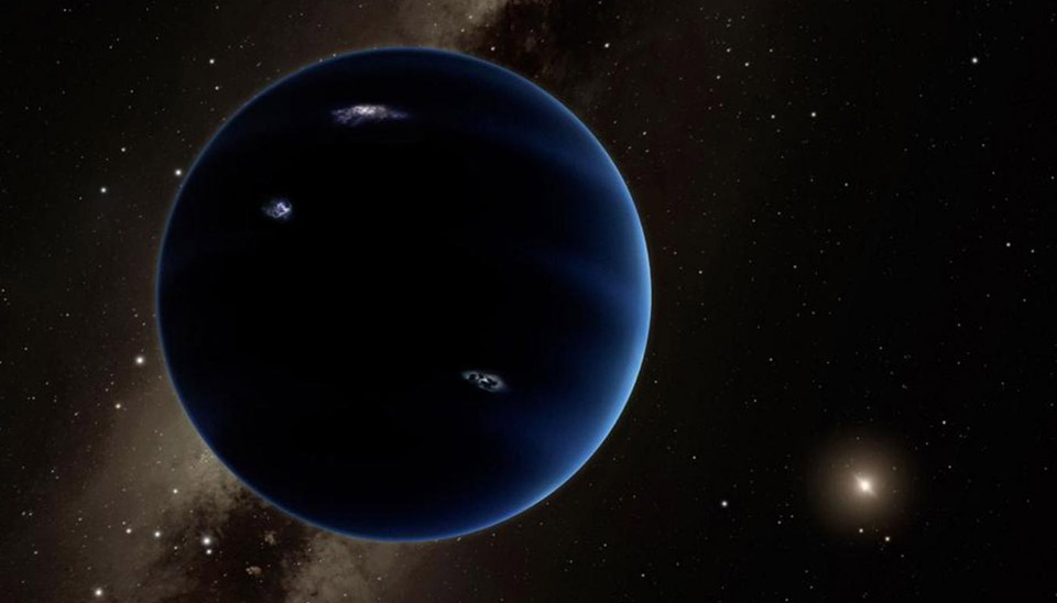
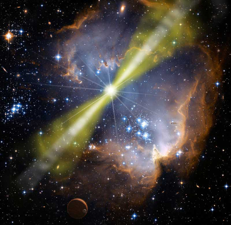
Artist’s illustration of Planet Nine, a hypothesized Neptune-sized planet orbiting in the distant reaches of our solar system. [Caltech/Robert Hurt]

What is Planet Nine?

In January of this year, Caltech researchers Konstantin Batygin and Mike Brown presented evidence of a distant ninth planet in our solar system. They predicted this planet to be of a mass and volume consistent with a super-Earth, orbiting on a highly eccentric path with a period of tens of thousands of years.

Since Batygin and Brown’s prediction, scientists have been hunting for further signs of Planet Nine. Though we haven’t yet discovered an object matching its description, we have come up with new strategies for finding it, we set some constraints on where it might be, and we made some interesting theoretical predictions about its properties.

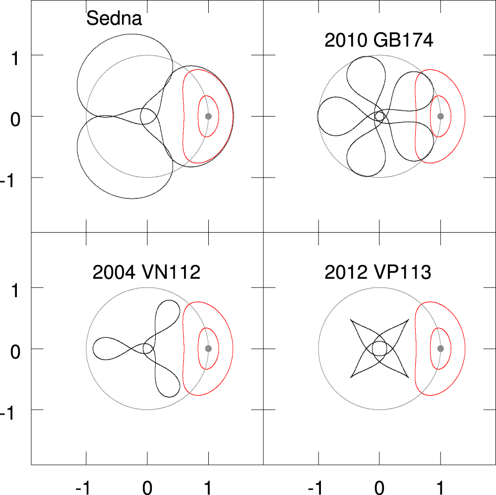
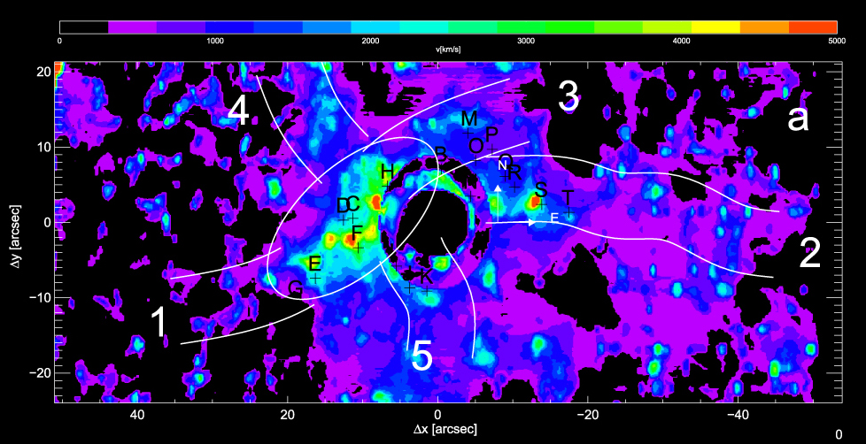
Visualizations of the resonant orbits of the four longest-period Kuiper belt objects, depicted in a frame rotating with the mean angular velocity of Planet Nine. Planet Nine’s position is on the right (with the trace of possible eccentric orbits e=0.17 and e=0.4 indicated in red). [Malhotra et al 2016]

Here are some of the newest constraints on Planet Nine from studies published just within the past two weeks.

Resonant Orbits

Renu Malhotra (University of Arizona’s Lunar and Planetary Laboratory) and collaborators present further evidence of the shaping of solar system orbits by the hypothetical Planet Nine. The authors point out that the four longest-period Kuiper belt objects (KBOs) have orbital periods close to integer ratios with each other. Could it be that these outer KBOs have become locked into resonant orbits with a distant, massive body?

The authors find that a distant planet orbiting with a period of ~17,117 years and a semimajor axis ~665 AU would have N/1 and N/2 period ratios with these four objects. If this is correct, it significantly constrains the parameters of Planet Nine’s orbit — as well as where it currently could be within its orbit.

Eliminating Hiding Spots

Brown and Batygin have returned, this time with more detailed estimates of Planet Nine’s potential orbit and location. By performing an enormous suite of simulations and then comparing the outcomes to actual observations of the distribution of KBOs, the authors narrow the allowed range for Planet Nine’s orbital characteristics.

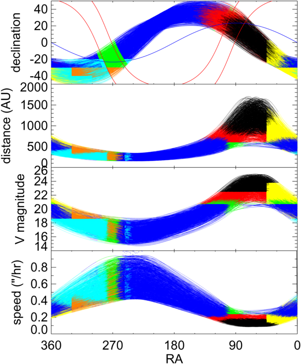
Authors’ predictions for the location, distance, brightness, and speed of Planet Nine throughout its orbit. Colored regions have been or will be explored by previous or current surveys capable of detecting the planet. Black regions remain places where Planet Nine could lurk. [Brown & Batygin 2016]

Brown and Batygin find that the allowed orbits for Planet Nine have perihelia of ~150–350 AU, semimajor axes of ~380–980 AU, and masses of ~5–20 Earth masses. Using these values and what we know about detection limits of previous and current surveys, we can rule out roughly two thirds of Planet Nine’s orbit, narrowing its position to be somewhere near aphelion.

Planet Nine’s Atmosphere

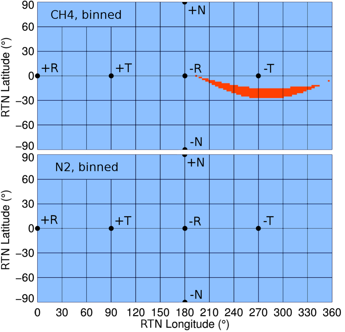
Finally, Jonathan Fortney (UC Santa Cruz) and collaborators model Planet Nine’s atmosphere. Rather than assuming the planet behaves like a blackbody, they use the planet’s predicted orbit — as well as a range of plausible masses and interior structures — in models that treat the body like the giant planets of our solar system.

The authors find Planet Nine is likely quite cold, as expected, with an effective temperature of ~35–50 K at most (for reference, Neptune is around 60 K). Because of this cool temperature, the authors speculate that methane may condense out of the atmosphere, changing the planet’s reflection and emission spectra. This would cause the planet to appear much “bluer” than planets like Uranus and Neptune in infrared energy bands.

The constraints from these studies continue to support the existence of Planet Nine, narrow down the regions in which we should search for it, and help us to better understand what signatures we’re looking for. In the words of Fortney et al., “Let the hunt continue.”

Citation

Renu Malhotra et al 2016 ApJ 824 L22. doi:10.3847/2041-8205/824/2/L22
Michael E. Brown and Konstantin Batygin 2016 ApJ 824 L23. doi:10.3847/2041-8205/824/2/L23
Jonathan J. Fortney et al 2016 ApJ 824 L25. doi:10.3847/2041-8205/824/2/L25

22 June 2016

Mapping Near-Earth Hazards

How can we hunt down all the near-Earth asteroids that are capable of posing a threat to us? A new study looks at whether the upcoming Large Synoptic Survey Telescope (LSST) is up to the job.

Charting Nearby Threats

LSST is an 8.4-m wide-survey telescope currently being built in Chile. When it goes online in 2022, it will spend the next ten years surveying our sky, mapping tens of billions of stars and galaxies, searching for signatures of dark energy and dark matter, and hunting for transient optical events like novae and supernovae. But in its scanning, LSST will also be looking for asteroids that approach near Earth.

Cumulative number of near-Earth asteroids discovered over time, as of June 16, 2016. [NASA/JPL/Chamberlin]

Near-Earth objects (NEOs) have the potential to be hazardous if they cross Earth’s path and are large enough to do significant damage when they impact Earth. Earth’s history is riddled with dangerous asteroid encounters, including the recent Chelyabinsk airburst in 2013, the encounter that caused the kilometer-sized Meteor Crater in Arizona, and the impact thought to contribute to the extinction of the dinosaurs.

Recognizing the potential danger that NEOs can pose to Earth, Congress has tasked NASA with tracking down 90% of NEOs larger than 140 meters in diameter. With our current survey capabilities, we believe we’ve discovered roughly 25% of these NEOs thus far. Now a new study led by Tommy Grav (Planetary Science Institute) examines whether LSST will be able to complete this task.

Absolute magnitude, H, of a synthetic NEO population. Though these NEOs are all larger than 140 m, they have a large spread in albedos. [Grav et al. 2016]

Can LSST Help?

Based on previous observations of NEOs and resulting predictions for NEO properties and orbits, Grav and collaborators simulate a synthetic population of NEOs all above 140 m in size. With these improved population models, they demonstrate that the common tactic of using an asteroid’s absolute magnitude as a proxy for its size is a poor approximation, due to asteroids’ large spread in albedos. Roughly 23% of NEOs larger than 140 m have absolute magnitudes fainter than H = 22 mag, the authors show — which is the value usually assumed as the default absolute magnitude of a 140 m NEO.

$NEO fraction detectable$

Fraction of NEOs we’ve detected as a function of time based on the authors’ simulations of the current surveys (red), LSST plus the current surveys (black), NEOCam plus the current surveys (blue), and the combined result for all surveys (green). [Grav et al. 2016]

Taking this into account, Grav and collaborators then use information about the planned LSST survey strategies and detection limits to test what fraction of this synthetic NEO population LSST will be able to detect in its proposed 10-year mission.

The authors find that, within 10 years, LSST will likely be able to detect only 63% of NEOs larger than 140 m. Luckily, LSST may not have to work alone; in addition to the current surveys in operation, a proposed infrared space-based survey mission called NEOCam is planned for launch in 2021. If NEOCam is funded, it will complement LSST’s discovery capabilities, potentially allowing the two surveys to jointly achieve the 90% detection goal within a decade.

Citation

T. Grav et al 2016 AJ 151 172. doi:10.3847/0004-6256/151/6/172

10 June 2016

Jets from Merging Neutron Stars

With the recent discovery of gravitational waves from the merger of two black holes, it’s especially important to understand the electromagnetic signals resulting from mergers of compact objects. New simulations successfully follow a merger of two neutron stars that produces a short burst of energy via a jet consistent with short gamma-ray burst (sGRB) detections.

Still from the authors’ simulation showing the two neutron stars, and their magnetic fields, before merger. [Adapted from Ruiz et al. 2016]

Challenging System

We have long suspected that sGRBs are produced by the mergers of compact objects, but this model has been difficult to prove. One major hitch is that modeling the process of merger and sGRB launch is very difficult, due to the fact that these extreme systems involve magnetic fields, fluids and full general relativity.

Traditionally, simulations are only able to track such mergers over short periods of time. But in a recent study, Milton Ruiz (University of Illinois at Urbana-Champaign and Industrial University of Santander, Colombia) and coauthors Ryan Lang, Vasileios Paschalidis and Stuart Shapiro have modeled a binary neutron star system all the way through the process of inspiral, merger, and the launch of a jet.

A Merger Timeline

How does this happen? Let’s walk through one of the team’s simulations, in which dipole magnetic field lines thread through the interior of each neutron star and extend beyond its surface (like magnetic fields found in pulsars). In this example, the two neutron stars each have a mass of 1.625 solar masses.

Simulation start (0 ms)
Loss of energy via gravitational waves cause the neutron stars to inspiral.
Merger (3.5 ms)
The neutron stars are stretched by tidal effects and make contact. Their merger produces a hypermassive neutron star that is supported against collapse by its differential (nonuniform) rotation.
Delayed collapse into a black hole (21.5 ms)
Once the differential rotation is redistributed by magnetic fields and partially radiated away in gravitational waves, the hypermassive neutron star loses its support and collapses to a black hole.
Plasma velocities turn around (51.5 ms)
Initially the plasma was falling inward, but as the disk of neutron-star debris is accreted onto the black hole, energy is released. This turns the plasma near the black hole poles around and flings it outward.
Magnetic field forms a helical funnel (62.5 ms)
The fields near the poles of the black hole amplify as they are wound around, creating a funnel that provides the wall of the jet.
Jet outflow extends to heights greater than 445 km (64.5 ms)
The disk is all accreted and, since the fuel is exhausted, the outflow shuts off (within 100ms)

Neutron-Star Success

Plot showing the gravitational wave signature for one of the authors’ simulations. The moments of merger of the neutron stars and collapse to a black hole are marked. [Adapted from Ruiz et al. 2016]

These simulations show that no initial black hole is needed to launch outflows; a merger of two neutron stars can result in an sGRB-like jet. Another interesting result is that the magnetic field configuration doesn’t affect the formation of a jet: neutron stars with magnetic fields confined to their interiors launch jets as effectively as those with pulsar-like magnetic fields. The accretion timescale for both cases is consistent with the duration of an sGRB.

While this simulation models milliseconds of real time, it’s enormously computationally challenging and takes months to simulate. The successes of this simulation represent exciting advances in numerical relativity, as well as in our understanding of the electromagnetic counterparts that may accompany gravitational waves.

Bonus

Check out this awesome video of the authors’ simulations. The colors differentiate the plasma density and the white lines depict the pulsar-like magnetic field that initially threads the two merging neutron stars. Watch as the neutron stars evolve through the different stages outlined above, eventually forming a black hole and launching a powerful jet. [Simulations and visualization by M. Ruiz, R. Lang, V. Paschalidis, S. Shapiro and the Illinois Relativity Group REU team: S. Connelly, C. Fan, A. Khan, and P. Wongsutthikoson]

Citation

Milton Ruiz et al 2016 ApJ 824 L6. doi:10.3847/2041-8205/824/1/L6

8 June 2016

Cold Accretion from the Cosmic Web

The cosmic web is a vast, foam-like network of filaments and voids stretching throughout the universe. How did the first galaxies form within the cosmic web, at the intersections of filaments? New observations of a “protodisk” — a galaxy in the early stages of formation — may provide a clue.

Models for Galaxy Formation

Narrowband image of the candidate protodisk (marked with a white ellipse) and filaments (outlined in white). [Adapted from Martin et al. 2016]

The standard model for galaxy formation, known as the “hot accretion model,” argues that galaxies form out of collapsing, virialized gas that forms a hot halo and then slowly cools, fueling star and galaxy formation at its center.

But what if galaxies are actually formed from cool gas? In this contrasting picture, the “cold accretion model,” cool (temperature of ~10⁴ K) unshocked gas from cosmic web filaments flows directly onto galactic disks forming at the filamentary intersections. The narrow streams of cold gas deliver fuel for star formation.

A signature of the cold accretion model is that the streams of cold gas form a disk as the gas spirals inward, sinking toward the central protogalaxy. Detecting these “cold-flow disks” could be strong evidence in support of this model — and last year, a team of authors reported just such a detection! This year they’re back again with a second object that may provide confirmation of cold accretion from the cosmic web.

A Candidate Protodisk

The team, led by Christopher Martin (California Institute of Technology), made the discovery using the Palomar Cosmic Web Imager, an instrument designed to observe faint emission from the intergalactic medium. Martin and collaborators found a large (R > 100 kpc, more than six times the radius of the Milky Way), rotating structure of hydrogen gas, illuminated by the nearby quasi-stellar object QSO HS1549+1919. The system is located at a redshift of z~2.8.

Three potential kinematic models of the candidate protodisk and filaments. a) Two filaments feed the disk, b) one filament feeds the disk, seen at 1.5 Gyr, and c) same as b, but after only 1.1 Gyr. [Martin et al. 2016]

The authors test three potential kinematic models of the candidate protodisk and filaments. In (a) two filaments feed the disk, in (b) one filament feeds the disk, seen at 1.5 Gyr, and (c) is the same as (b), but after only 1.1 Gyr. [Martin et al. 2016]

This protodisk, which they characterize based on the distribution and velocity of gas within it, appears to be being fed by one or possibly more filaments. Martin and collaborators analyze and model the disk and its accretion flows, and show that the observed protodisk was likely formed recently, and the gas flowing onto it is low-metallicity, probably coming directly from the cosmic web.

This protodisk is very similar to the group’s previous discovery of a disk illuminated by QSO UM287. Their new discovery of a second such protodisk suggests that these objects may be common, and it confirms that cold-flow accretion is present at these redshifts. Searching for more of these objects will help us to better understand the specifics of how galaxies form from the cosmic web.

Citation

D. Christopher Martin et al 2016 ApJ 824 L5. doi:10.3847/2041-8205/824/1/L5

6 June 2016

Testing Our Fundamental Assumptions

Science is all about testing the things we take for granted — including some of the most fundamental aspects of how we understand our universe. Is the speed of light in a vacuum the same for all photons regardless of their energy? Is the rest mass of a photon actually zero? A series of recent studies explore the possibility of using transient astrophysical sources for tests!

Explaining Different Arrival Times

Artist’s illustration of a gamma-ray burst, another extragalactic transient, in a star-forming region. [NASA/Swift/Mary Pat Hrybyk-Keith and John Jones]

Suppose you observe a distant transient astrophysical source — like a gamma-ray burst, or a flare from an active nucleus — and two photons of different energies arrive at your telescope at different times. This difference in arrival times could be due to several different factors, depending on how deeply you want to question some of our fundamental assumptions about physics:

Intrinsic delay
The photons may simply have been emitted at two different times by the astrophysical source.
Delay due to Lorentz invariance violation
Perhaps the assumption that all massless particles (even two photons with different energies) move at the exact same velocity in a vacuum is incorrect.
Special-relativistic delay
Maybe there is a universal speed for massless particles, but the assumption that photons have zero rest mass is wrong. This, too, would cause photon velocities to be energy-dependent.
Delay due to gravitational potential
Perhaps our understanding of the gravitational potential that the photons experience as they travel is incorrect, also causing different flight times for photons of different energies. This would mean that Einstein’s equivalence principle, a fundamental tenet of general relativity (GR), is incorrect.

If we now turn this problem around, then by measuring the arrival time delay between photons of different energies from various astrophysical sources — the further away, the better — we can provide constraints on these fundamental assumptions.

A recent focus set in the Astrophysical Journal Letters, titled “Focus on Exploring Fundamental Physics with Extragalactic Transients,” consists of multiple published studies doing just that.

Testing General Relativity

Several of the articles focus on the 4th point above. By assuming that the delay in photon arrival times is only due to the gravitational potential of the Milky Way, these studies set constraints on the deviation of our galaxy’s gravitational potential from what GR would predict. The study by He Gao et al. uses the different photon arrival times from gamma-ray bursts to set constraints at eV–GeV energies, and the study by Jun-Jie Wei et al. complements this by setting constraints at keV-TeV energies using photons from high-energy blazar emission.

Photons or neutrinos from different extragalactic transients each set different upper limits on delta gamma, the post-Newtonian parameter, vs. particle energy or frequency. This is a test of Einstein’s equivalence principle: if the principle is correct, delta gamma would be exactly zero, meaning that photons of different energies move at the same velocity through a vacuum. [Tingay & Kaplan 2016]

S.J. Tingay & D.L. Kaplan make the case that measuring the time delay of photons from fast radio bursts (FRBs; transient radio pulses that last only a few milliseconds) will provide even tighter constraints — if we are able to accurately determine distances to these FRBs.

And Adi Musser argues that the large-scale structure of the universe plays an even greater role than the Milky Way gravitational potential, allowing for even stricter testing of Einstein’s equivalence principle.

The ever-narrower constraints from these studies all support GR as a correct set of rules through which to interpret our universe.

Other Tests of Fundamental Physics

In addition to the above tests, Xue-Feng Wu et al. show that FRBs can be used to provide severe constraints on the rest mass of the photon, and S. Croft et al. even touches on what we might learn from transients using multi-messenger astrophysics (astrophysics involving observations of particles besides photons, such as neutrinos or gravitational waves).

In general, extragalactic transients provide a rich prospect for better understanding the laws that govern the universe. Check out the entire focus set below to learn more about the tests of fundamental physics that can be done with observations of extragalactic transients!

Citation

Focus Set: Focus on Exploring Fundamental Physics With Extragalactic Transients

He Gao et al. 2015 ApJ 810 121. doi:10.1088/0004-637X/810/2/121
Jun-Jie Wei et al. 2016 ApJ 818 L2. doi:10.3847/2041-8205/818/1/L2
S. Croft et al. 2016 ApJ 820 L24. doi:10.3847/2041-8205/820/2/L24
S. J. Tingay and D. L. Kaplan 2016 ApJ 820 L31. doi:10.3847/2041-8205/820/2/L31
Adi Nusser 2016 ApJ 821 L2. doi:10.3847/2041-8205/821/1/L2
Xue-Feng Wu et al. 2016 ApJ 822 L15. doi:10.3847/2041-8205/822/1/L15

25 May 2016

Clues From Pluto’s Ions

Nearly a year ago, in July 2015, the New Horizons spacecraft passed by the Pluto system. The wealth of data amassed from that flyby is still being analyzed — including data from the Solar Wind Around Pluto (SWAP) instrument. Recent examination of this data has revealed interesting new information about Pluto’s atmosphere and how the solar wind interacts with it.

A Heavy Ion Tail

The solar wind is a constant stream of charged particles released by the Sun at speeds of around 400 km/s (that’s 1 million mph!). This wind travels out to the far reaches of the solar system, interacting with the bodies it encounters along the way.

By modeling the SWAP detections, the authors determine the directions of the IMF that could produce the heavy ions detected. Red pixels represent IMF directions permitted. No possible IMF could reproduce the detections if the ions are nitrogen (bottom panels), and only retrograde IMF directions can produce the detections if the ions are methane. [Adapted from Zirnstein et al. 2016]

New Horizons data has revealed that Pluto’s atmosphere leaks neutral nitrogen, methane, and carbon monoxide molecules that sometimes escape its weak gravitational pull. These molecules become ionized and are subsequently “picked up” by the passing solar wind, forming a tail of heavy ions behind Pluto. The details of the geometry and composition of this tail, however, had not yet been determined.

Escaping Methane

In a recent study led by Eric Zirnstein (Southwest Research Institute), the latest analysis of data from the SWAP instrument on board New Horizons is reported. The team used SWAP’s ion detections from just after New Horizons’ closest approach to Pluto to better understand how the heavy ions around Pluto behave, and how the solar wind interacts with Pluto’s atmosphere.

In the process of analyzing the SWAP data, Zirnstein and collaborators first establish what the majority of the heavy ions picked up by the solar wind are. Models of the SWAP detections indicate they are unlikely to be nitrogen ions, despite nitrogen being the most abundant molecule in Pluto’s atmosphere. Instead, the detections are likely of methane ions — possibly present because methane molecules are lighter, allowing them to more efficiently escape Pluto’s atmosphere.

Reconstructed origins of heavy ions detected by SWAP shortly after New Horizons’ closest approach to Pluto. Color represents the energy at the time of detection. [Adapted from Zirnstein et al. 2016]

Magnetic Direction

New Horizons does not have a magnetometer on board, which prevented it from making direct measurements of the interplanetary magnetic field (IMF; the solar magnetic field extended throughout the solar system) during the Pluto encounter. In spite of this, Zirnstein and collaborators are able to determine the IMF direction using some clever calculations about SWAP’s field of view and the energies of heavy ions it detected.

They demonstrate that the IMF was likely oriented roughly parallel to the ecliptic plane, and in the opposite direction of Pluto’s orbital motion, during New Horizon’s Pluto encounter. This would cause the solar wind to deflect southward around Pluto, resulting in a north-south asymmetry in the heavy ion tail behind Pluto.

The new knowledge gained from SWAP about the geometry and the composition of Pluto’s extended atmosphere will help us to interpret further data from New Horizons. Ultimately, this provides us with a better understanding both of Pluto’s atmosphere and how the solar wind interacts with bodies in our solar system.

Citation

E. J. Zirnstein et al 2016 ApJ 823 L30. doi:10.3847/2041-8205/823/2/L30

23 May 2016

A Comet’s Missing Light

On 28 November 2013, comet C/2012 S1 — better known as comet ISON — should have passed within two solar radii of the Sun’s surface as it reached perihelion in its orbit. But instead of shining in extreme ultraviolet (EUV) wavelengths as it grazed the solar surface, the comet was never detected by EUV instruments. What happened to comet ISON?

Missing Emission

When a sungrazing comet passes through the solar corona, it leaves behind a trail of molecules evaporated from its surface. Some of these molecules emit EUV light, which can be detected by instruments on telescopes like the space-based Solar Dynamics Observatory (SDO).

Comet ISON, a comet that arrived from deep space and was predicted to graze the Sun’s corona in November 2013, was expected to cause EUV emission during its close passage. But analysis of the data from multiple telescopes that tracked ISON in EUV — including SDO — reveals no sign of it at perihelion.

In a recent study, Paul Bryans and Dean Pesnell, scientists from NCAR’s High Altitude Observatory and NASA Goddard Space Flight Center, try to determine why ISON didn’t display this expected emission.

Comparing ISON and Lovejoy

In December 2011, another comet dipped into the Sun’s corona: comet Lovejoy. This image, showing the orbit Lovejoy took around the Sun, is a composite of SDO images of the pre- and post-perihelion phases of the orbit. Click for a closer look! The dashed part of the curve represents where Lovejoy passed out of view behind the Sun. [Bryans & Pesnell 2016]

This is not the first time we’ve watched a sungrazing comet with EUV-detecting telescopes: Comet Lovejoy passed similarly close to the Sun in December 2011. But when Lovejoy grazed the solar corona, it emitted brightly in EUV. So why didn’t ISON? Bryans and Pesnell argue that there are two possibilities:

the coronal conditions experienced by the two comets were not similar, or
the two comets themselves were not similar.

To establish which factor is the most relevant, the authors first demonstrate that both comets experienced very similar radiation fields as they passed perihelion. They also show that the properties of the Sun’s corona experienced by each comet — like its density and magnetic field topology — were roughly the same.

Bryans and Pesnell argue that, as both comets appear to have encountered similar solar conditions, the most likely explanation for ISON’s lack of detectable EUV emission is that it didn’t deposit as much material in its orbit as Lovejoy did. They show that this would happen if ISON’s nucleus were four times smaller in radius than Lovejoy’s, spanning a mere 50–70 meters in comparison to Lovejoy’s 200–300 meters.

This conclusion is consistent with white-light observations of ISON that suggest that, though it might have started out significantly larger than Lovejoy, ISON underwent dramatic mass loss as it approached the Sun. By the time it arrived at perihelion, it was likely no longer large enough to create a strong EUV signal — resulting in the non-detection of this elusive comet with SDO and other telescopes.

Citation

Paul Bryans and W. Dean Pesnell 2016 ApJ 822 77. doi:10.3847/0004-637X/822/2/77

20 May 2016

Building Halos by Digesting Satellites

We think galactic halos are built through the addition of material from the smaller subhalos of satellites digested by their hosts. Though most of the stars in Milky-Way-mass halos were probably formed in situ, many were instead accumulated over time, as orbiting dwarf galaxies were torn apart and their stars flung throughout the host galaxy. A recent set of simulations has examined this brutal formation process.

In the authors’ simulations, a subhalo first falls into the host halo. At this point, it can either survive to present day as a satellite galaxy, or it can be destroyed, its stars scattering throughout the host halo. [Deason et al. 2016]

Subhalo Fate

There are many open questions about the growth of Milky-Way-mass halos from the accretion of subhalos. Which subhalos are torn apart and accreted, and which ones survive intact? Are more small or large subhalos accreted? Does subhalo accretion affect the host galaxy’s metallicity? And what can we learn from all of this about the Milky Way’s formation history?

In a recently published study, a team of scientists from Stanford University and SLAC National Accelerator Laboratory set out to answer these questions using a suite of 45 zoom-in simulations of Milky-Way-mass halos. Led by Alis Deason, the team tracked the accretion history of these 45 test galaxies to determine how their halos were built.

Piecing Together History

Deason and collaborators reach several new and interesting conclusions based on the outcomes of their simulations.

Average accreted stellar mass from destroyed dwarfs for each host halo, as a function of the time of the last major accretion event. More stellar mass is accreted in more recent accretion events. [Deason et al. 2016]
Most of the stellar mass accreted by the Milky-Way-mass halos typically comes from only one or two destroyed dwarfs. The accreted dwarfs are usually low-mass if they were accreted early on in the simulation (i.e., in the early universe), and high-mass if they were accreted recently.
Dwarfs destroyed and accreted early on are typically low-metallicity — as would be expected, since metallicity was lower in the early universe. Dwarfs accreted later in the simulation are typically higher metallicity. So host halos with recent accretion events are not only likely to have accreted more stellar mass, but also probably higher-metallicity stars.
Though ultra-faint, low-mass dwarfs have lower average metallicities than the larger classical dwarfs, classical dwarfs contribute more of the very metal-poor stars accreted by host halos (40-80%, compared to the 2-5% from ultra-faint dwarfs).
Halos that have relatively quiescent accretion histories tend to have lower-mass surviving dwarfs today.

A Transient Fossil?

This last point has interesting implications for our own galaxy. The Milky Way is generally though to have a quiescent formation history, and yet it contains two high-mass surviving dwarfs: the Large and Small Magellanic Clouds. The authors suggest that this inconsistency could be resolved if the Milky Way is a “transient fossil” — a halo with a quiescent formation history masked by its recent acquisition of the Large and Small Magellanic Clouds.

The outcomes from this suite of simulations provide important clues for better understanding how our own galaxy — and galaxies like ours — have formed and evolved.

Citation

Alis J. Deason et al 2016 ApJ 821 5. doi:10.3847/0004-637X/821/1/5

18 May 2016

Reconnection on the Sun

Because the Sun is so close, it makes an excellent laboratory to study processes we can’t examine in distant stars. One open question is that of how solar magnetic fields rearrange themselves, producing the tremendous releases of energy we observe as solar flares and coronal mass ejections (CMEs).

What is Magnetic Reconnection?

Magnetic reconnection occurs when a magnetic field rearranges itself to move to a lower-energy state. As field lines of opposite polarity “reconnect”, magnetic energy is suddenly converted into thermal and kinetic energy.

This process is believed to be behind the sudden releases of energy from the solar surface in the form of solar flares and CMEs. But there are many different models for how magnetic reconnection could occur in the magnetic field at the Sun’s surface, and we aren’t sure which one of these reconnection types is responsible for the events we see.

Recently, however, several studies have been published presenting some of the first observational support of specific reconnection models. Taken together, these observations suggest that there are likely several different types of reconnection happening on the solar surface. Here’s a closer look at two of these recent publications:

A pre-eruption SDO image of a flaring region (b) looks remarkably similar to a 3D cartoon for typical breakout configuration (a). Click for a closer look! [Adapted from Chen et al. 2016]

Study 1: Magnetic Breakout

Led by Yao Chen (Shandong University in China), a team of scientists has presented observations made by the Solar Dynamics Observatory (SDO) of a flare and CME event that appears to have been caused by “magnetic breakout”.

In the magnetic breakout model, a series of loops in the Sun’s lower corona are confined by a surrounding larger loop structure — called an arcade — higher in the corona. As the lower loops push upward, reconnection occurs in the upper corona, removing the overlying, confining arcade. Without that extra confinement, the lower coronal loops expand upward, erupting from the solar surface.

Snapshots from the SDO side view (left and center) and STEREO overhead view (right). The three rows show the time evolution of the double-loop structure after the initial flare. In the STEREO view, you can see the central footpoints of the loops slip to the left. [Gou et al. 2016]

In the SDO observations presented by Chen and collaborators, the pre-flare/CME structures look remarkably like the structures predicted in the breakout model. Sequential heating of loops can be seen as the breakout reconnection starts, followed by an enormous flare and CME as the lower loops erupt outward.

Study 2: Slipping Reconnection

A team of scientists from the University of Science and Technology of China, led by Tingyu Gou and Rui Liu, have presented the first stereoscopic observation of “slipping reconnection” in the Sun, made by the two-spacecraft Solar Terrestrial Relations Observatory (STEREO).

In slipping reconnection, magnetic field lines continuously exchange connectivities with their neighbors, causing them to slip through plasma. Observations by STEREO of a flaring double-loop system revealed that the central footpoints — the endpoints where the loops are anchored to the solar surface — slipped sideways after a flare.

The authors’ model of the double-loop structure at two different times, during which the central footpoint slips from point C to D. Projections onto the XY and YZ planes show STEREO’s and SDO’s views, respectively. [Gou et al. 2016]

The authors reconstructed a 3D model of the loop system using the overhead observations from STEREO and a simultaneous side view from SDO. They speculate that the slipping reconnection was likely triggered by the initial solar flare.

Double Bonus

Check out the videos below to watch these processes happen!

This first video is from Chen et al. 2016, and shows the SDO view of coronal loops in three wavelengths. If you watch carefully, you can see the sequential brightening of loops — signs of the breakout reconnection — before the flare and CME.

This second video is from Gou et al. 2016, and shows the SDO side view (left and center panels) and STEREO top view (right panel) of a flare and the slipping reconnection that occurred after. Keep your eye on the STEREO view between 0:02 and 0:04 to watch the central footpoint slide left.

Citation

Yao Chen et al 2016 ApJ 820 L37. doi:10.3847/2041-8205/820/2/L37

Tingyu Gou et al 2016 ApJ 821 L28. doi:10.3847/2041-8205/821/2/L28

16 May 2016

Discovery of Methanol in a Planetary Birthplace

Data from the Atacama Large Millimeter/submillimeter Array (ALMA) has recently revealed the first detection of gas-phase methanol, a derivative of methane, in a protoplanetary disk. This milestone discovery is an important step in understanding the conditions for planet formation that can lead to life-supporting planets like Earth.

Planetary Chemistry

One major goal in the study of exoplanets is to find planets that orbit in their host stars’ habitable zones, a measure that determines whether the planet receives the right amount of sunlight to support liquid water. But there’s another crucial element in the formation of a life-supporting planet: chemistry.

To understand the chemistry of newly born planets, we need to study protoplanetary disks — because it’s from these that young planets form. The elements and molecules contained in these dusty disks are what initially make up the atmospheres of planets forming within the disks.

The Atacama Large Millimeter/submillimeter Array under the southern sky. [ESO/B. Tafreshi]

The Hunt for Complexity

The detection of complex molecules in protoplanetary disks is an important milestone, because complex molecules are necessary to build the correct chemistry to support life. Unfortunately, detecting these molecules is very difficult, requiring observations with both high spatial resolution and high sensitivity. Thus far, though we’ve observed elements and simple molecules in protoplanetary disks, detections of complex molecules have been elusive — with only one success before now.

Luckily, we now have an observatory up to the challenge! ALMA’s unprecedented spatial resolution and sensitivity has recently allowed a team of scientists led by Catherine Walsh (Leiden University) to observe gas-phase methanol in a protoplanetary disk for the first time. This detection was made in the disk around the young star TW Hya, and it represents one of the largest molecules that has ever been observed in a disk to date.

Locating Ices

The model (purple line) and data (dashed line) showing the methanol line detection. [Adapted from Walsh et al. 2016]

Since TW Hya’s disk has temperatures of less than ~100K (-173°C), we would expect most of the disk’s methanol to be frozen. The gas-phase methanol observed by Walsh and collaborators was likely released from a larger reservoir of frozen methanol residing on dust grains in the disk. The peak of the methanol emission was detected from a ring located about 30 AU out from the central star, which suggests that the larger dust grains in the disk — located in the inner 50 AU — may host the bulk of the disk ice reservoir.

Walsh and collaborator’s important detection opens a window into studying complex organic chemistry during planetary system formation. This stepping stone can help us to better understand the conditions when Earth formed and what we should look for in the search for life-supporting planets.

Citation

Catherine Walsh et al 2016 ApJ 823 L10. doi:10.3847/2041-8205/823/1/L10

Previous 1 … 105 106 107 108 109 … 118 Next