Astrobites Archives - Page 3 of 46

Astrobites RSS

18 July 2025

Written in the Gas: Jet Feedback in a Voorwerp Galaxy

Title: Jet-Mode Feedback in NGC 5972: Insights from Resolved MUSE, GMRT, and VLA Observations
Authors: Arshi Ali et al.
First Author’s Institution: Savitribai Phule Pune University
Status: Published in ApJ

Voorwerp Galaxies as Laboratories for Active Galactic Nuclei

Supermassive black holes are believed to reside at the centers of nearly all massive galaxies. As supermassive black holes accrete matter, they can release enormous amounts of energy in the form of radiation, winds, and relativistic jets — powering active galactic nuclei and influencing their host galaxies. This process, known as active galactic nucleus feedback, can regulate star formation and the properties of the gas in the interstellar medium, making it a key mechanism for shaping how galaxies form and evolve over cosmic time.

Of the many diverse manifestations of active galactic nuclei, radio “loud” galaxies stand out as powerful laboratories for studying feedback in action. Not only do these galaxies have characteristic [O III] emission lines, but they also host intense radio-emitting lobes of gas that extend well beyond the structure of the galaxy, indicative of jets. (Today’s article refers to these lobes as the extended emission-line region or EELR.)

Originally discovered by a schoolteacher, Voorwerp galaxies are a special category of radio galaxies that are candidate sites of active galactic nucleus activity in terms of their emission-line signatures. Moreover, they exhibit intriguing clouds of ionized gas that may have originated from jets. Figure 1 shows some examples of Voorwerp galaxies. Exploring these galaxies can shed light on how jets interact with the interstellar medium, a major player in active galactic nucleus feedback.

Figure 1: Voorwerp galaxies are compelling laboratories for exploring the interaction between jets and the interstellar medium. Examples are Hanny’s Voorwerp (left), NGC 5972 (middle), and the Teacup Quasar (right). [NASA, ESA, W. Keel (University of Alabama), and the Galaxy Zoo Team; NASA, ESA, and W. Keel (University of Alabama, Tuscaloosa); NASA, ESA, and W. Keel (University of Alabama, Tuscaloosa)]

Today’s article focuses on the physical and kinematic properties of one particular Voorwerp galaxy, NGC 5972. This galaxy is interesting for its bizarre, helical structure of ionized gas, as well as hints of a rich history of active galactic nucleus activity. Could jet feedback have played a significant role in the evolution of this galaxy?

Evidence for Relativistic Jets in NGC 5972

To study the interstellar medium of the Voorwerp galaxy, the authors combined observations from multiple instruments that probe different phases of the galaxy’s gas. Specifically, they used data from the Very Large Telescope (VLT), the Giant Metrewave Radio Telescope (GMRT), and the Very Large Array (VLA) to create maps of the ionized gas emission, allowing them to trace the structures and movement of the gas and jet material. Together, these datasets offer a comprehensive, multi-wavelength view of how the radio jet shaped the surrounding interstellar medium. The maps of NGC 5972, shown in Figure 2, display an impressive spiraling structure that could be the result of prolonged active galactic nucleus activity.

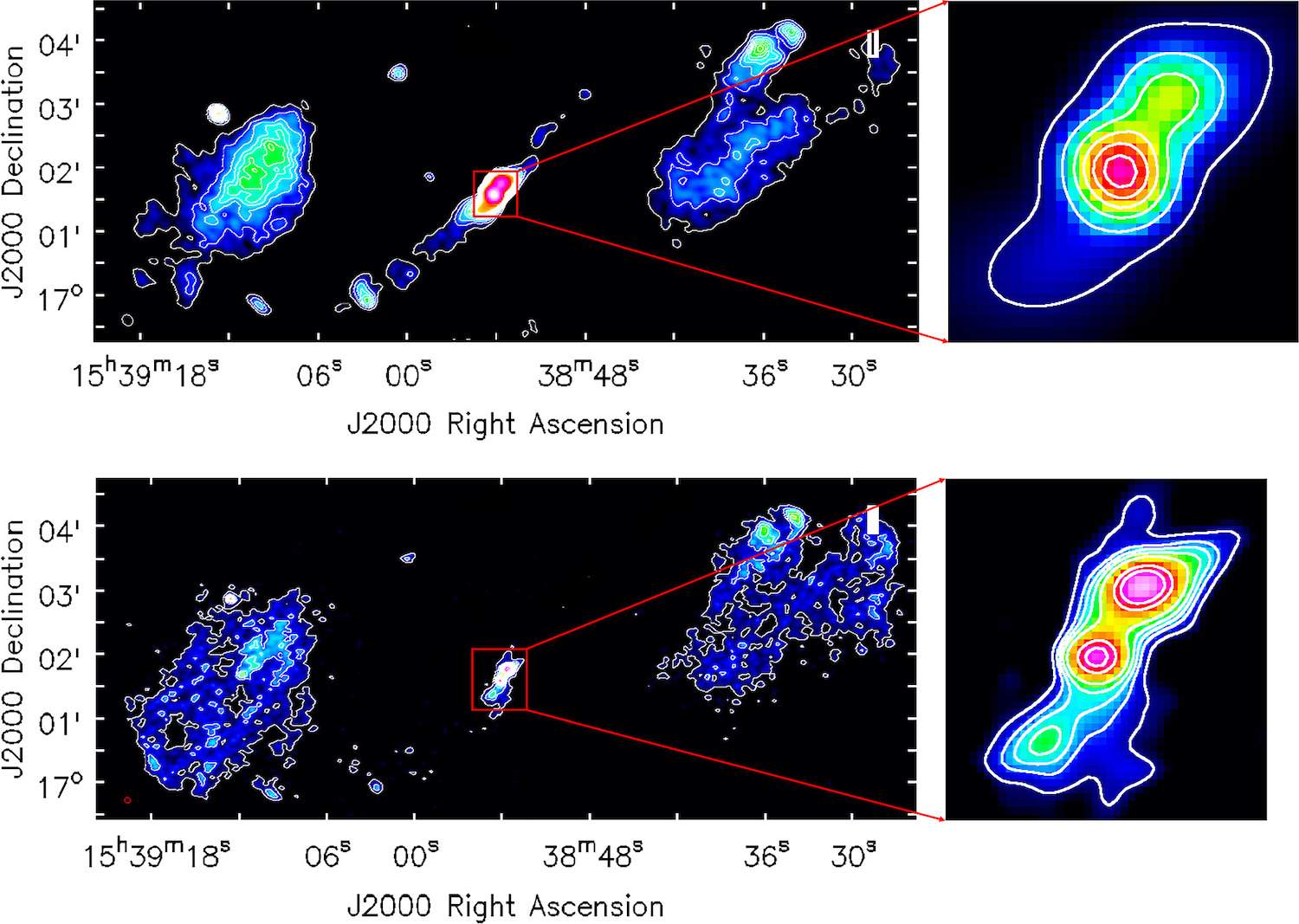
Figure 2: The radio emission of NGC 5972 reveals the extended helical, spiral structure of the ionized gas, where the inner jets are connected to the outer lobes (top: VLA, bottom: GMRT). This suggests that the intriguing shape of NGC 5972 could have originated from active galactic nucleus jets. [Ali et al. 2025]

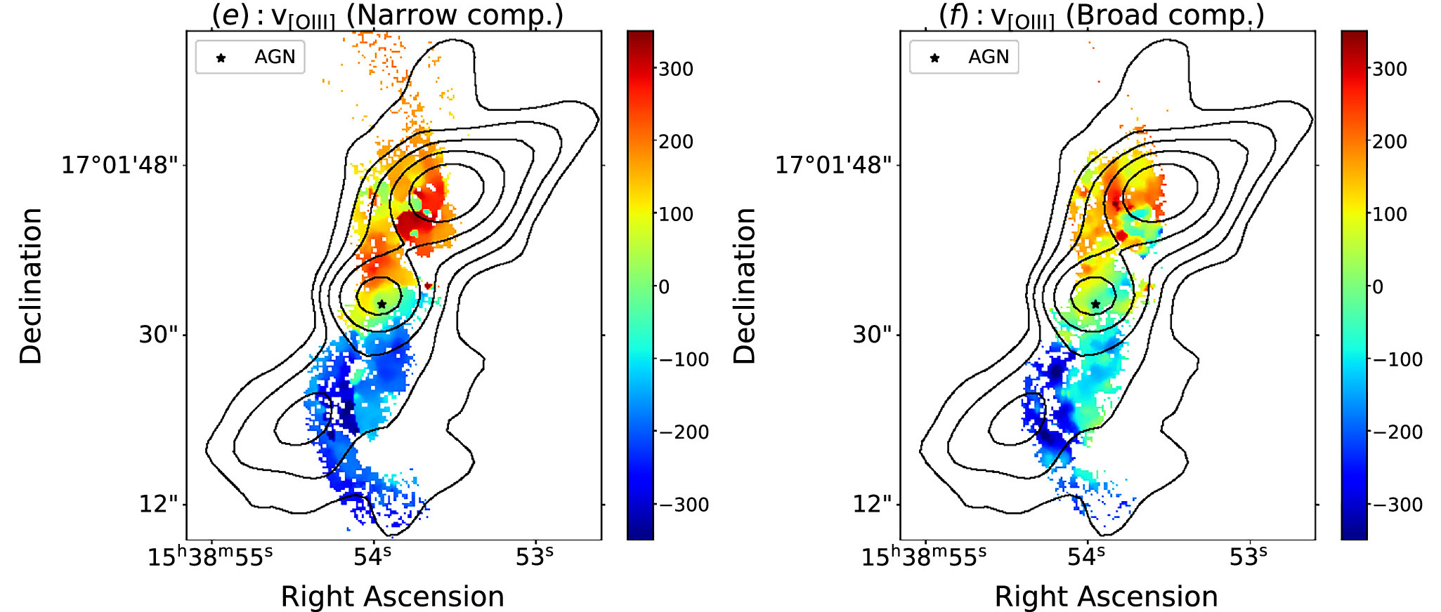
When the authors examined the extended emission-line region, they found that the velocity profiles (shown in Figure 3) are closely aligned with the direction of where we would expect to find a radio jet. The enhanced velocities around the jet region likely represent gas that is outflowing due to feedback. The expected amount of energy from a radio jet would have been capable of driving outflows at these velocities.

velocity profiles of the OIII emission lines

Figure 3: The velocity profiles of NGC 5972’s [O III] emission lines, a characteristic signature of the active galactic nucleus’s extended emission-line region. The velocities are aligned and enhanced along the jet axis, indicating that active galactic nucleus feedback influenced the gas by powering jets and outflows. [Adapted from Ali et al. 2025]

While the structure and movement of the ionized gas give promising hints of jet feedback, astronomers use a tool called Baldwin–Phillips–Terlevich (BPT) analysis to figure out what exactly is ionizing the gas. By comparing the ratio of different emission lines, we can categorize whether the galaxy’s gas was primarily ionized by radiation from an active galactic nucleus, stars, or other processes. The results of the BPT analysis are shown in the left panel of Figure 4.

Figure 4: The left panel shows the ionizing sources of the gas in NGC 5972. While the gas along the jet axis is ionized by radiation from the active galactic nucleus (orange in the diagram), the regions transverse to the jet are ionized by shock waves (blue). Moreover, the gas in the jet regions is more turbulent, as shown in the right panel. [Adapted from Ali et al. 2025]

In the case of NGC 5972, the radio jet is mostly ionized by radiation from the active galactic nucleus! However, the gas perpendicular to the jet shows a different signature — one that matches shock waves rather than strong radiation. In addition, the gas in the shock region is more turbulent (right panel of Figure 4). This suggests that the radio jet is not just a byproduct of the active galactic nucleus — it actively disturbs and heats the surrounding gas by way of shocks. This dual process of jet-induced shocks creates a richer picture of how supermassive black holes interact with the interstellar medium.

Putting the Story of NGC 5972 Together

These findings suggest that jet-driven feedback plays a crucial role in shaping the extended emission-line region of NGC 5972 (see Figure 5 for a summary). The interaction between the radio jet and the surrounding gas not only sustains ionization but also influences the gas structure. To further unravel the jet’s impact, future high-resolution radio observations will be essential, providing deeper insights into how active galactic nucleus–driven jets function.

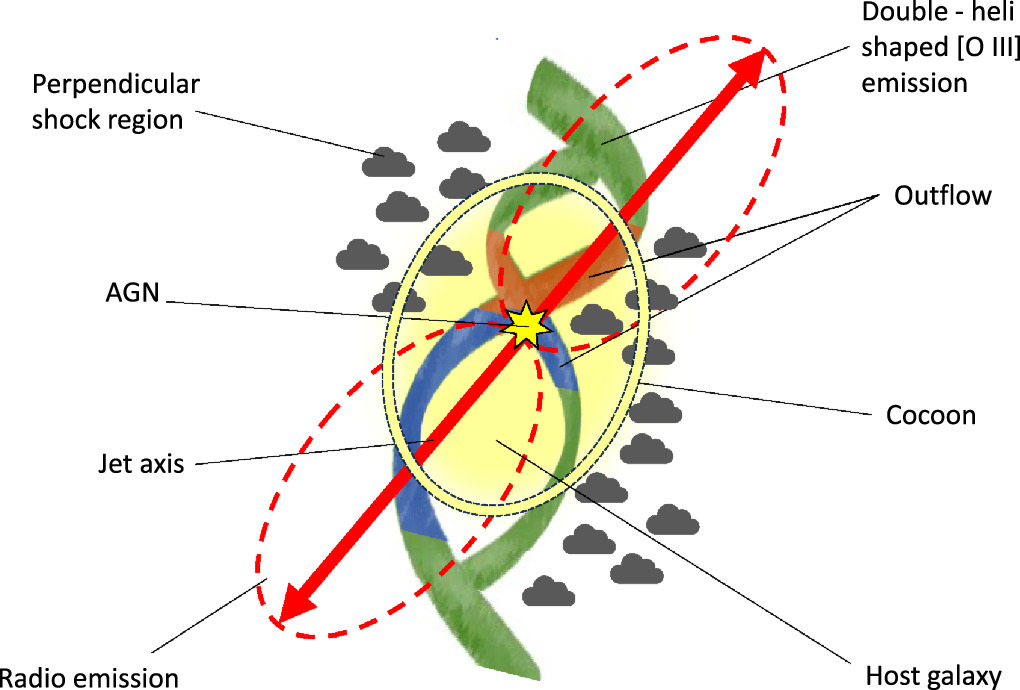
Figure 5: Cartoon schematic diagram showing various mechanisms at play in NGC 5972, including the active galactic nucleus jets, shocks, and outflows. [Ali et al. 2025]

NGC 5972 is more than just a bizarre-looking galaxy — it’s a time capsule, preserving the memory of a powerful supermassive black hole and revealing how its energy continues to shape the galaxy.

Original astrobite edited by Alexandra Masegian.

8 July 2025

You Shall Not Pass! Active Galactic Nucleus Jets Through the Interstellar Medium

Title: You Shall Not Pass! The Propagation of Low-/Moderate-Powered Jets Through a Turbulent Interstellar Medium
Authors: Olga Borodina et al.
First Author’s Institution: Center for Astrophysics | Harvard & Smithsonian
Status: Published in ApJ

The central black holes of some galaxies are surrounded by accretion disks of hot infalling gas. In cases when the accretion disk is massive and highly energetic, this central system forms an active galactic nucleus that outshines the rest of the galaxy. Active galactic nucleus feedback is the process of energetic interactions between the central supermassive black hole and its surroundings. Active galactic nuclei are essential for galaxy quenching, and correctly modeling their contribution is important for accurate cosmological simulations.

Active galactic nuclei release the energy from their accretion via winds, which are widespread outflows, and jets. Jets are collimated, fast outflows of baryonic matter that can spread out from hundreds to tens of thousands of parsecs from their origin. There’s a big range in power for jets, ranging from a low end of around 10³⁸ erg/s to a high end of 10⁴⁶ erg/s. For context, our Sun emits at about 10³³ erg/s.

As jets pass through their host galaxy, they interact with the gas and dust of the interstellar medium. There isn’t a lot of observational evidence for what goes on in that interaction, as the scale of resolution needed is so small — on the order of parsecs within the galaxy. Cosmological simulations don’t model scales small enough to accurately simulate these interactions, and they instead rely on feedback models that implement the macroscale effects. This means we could be missing part of the picture. Today’s article considers galaxy-scale numeric models for jets passing through a turbulent interstellar medium to study how the jet is affected by the gas and dust.

To do this, the authors used the Arepo code, which has an adaptive mesh setup that improves the resolution in areas that need it. They set up a 2-kiloparsec-cubed box full of gas with properties based on real galaxies’ interstellar media. This study is unique compared to other works because the authors use a filamentary structure for the interstellar medium, while previous studies used a clumpy structure. This filamentary structure reflects our actual Milky Way’s interstellar medium and creates more low-density cavities for the jet to interact with. The authors studied three jet powers on the low to intermediate end, of 10³⁸, 10⁴⁰, and 10⁴³ erg/s. This is also unique to the study, as many works look at higher-powered jets, which produce large-scale radio galaxies, despite lower powers being more common. The jets were launched along the x-axis and had a tracer set up to track their positions through time.

propagation of jets into the interstellar medium

Figure 1: From top to bottom, the high to low power jets, which are traced in color against the background interstellar medium density in grayscale. The lower power jets are stalled by the interstellar medium and do not make it as far out in the simulation space. [Adapted from Borodina et al. 2025]

This study found three different outcomes for the three jet powers (see Figure 1), and these general conclusions held up even when the authors changed the initial randomized structure of the interstellar medium.

The highest-power jets, 10⁴³ erg/s, were easily able to pass through the turbulent environment and reach the outer boundary of the simulation. They mostly traveled along the axis that the jet was launched along, with some lateral expansion.

The intermediate-power jets, 10⁴⁰ erg/s, were highly disrupted and redirected from the axis they were launched along. The jets bent, filled the low-density cavities between the filaments, and produced bubble-like shapes. These jets did make it all the way to the simulation boundary, but at later times and not along the axis they were initialized on. These intermediate-power jets don’t have enough ram pressure — the pressure against the gas due to the jet’s motion — to push through the turbulent structure of the interstellar medium, and they have to fill pre-existing cavities rather than plowing their own. The authors developed an analytic model for the minimum energy needed for jets to be able to plow through the interstellar medium, at approximately 10⁴¹ erg/s.

The jets in the lowest-power case, 10³⁸ erg/s, were stalled out by the interstellar medium within the first kiloparsec of travel. They couldn’t penetrate the higher-density regions of the interstellar medium the way the 10⁴⁰ erg/s case could, and they couldn’t make it to lower-density cavities to expand into.

All three of these cases were slower and shorter than the same power of jets run in a non-turbulent simulation, with the most significant disruption in the lowest-powered jets. This work demonstrates that a turbulent interstellar medium–jet interaction can be the sole cause of observed asymmetric and bent active galactic nucleus jets. By improving our understanding of this small-scale interaction, the authors are contributing to making better active galactic nucleus feedback models in cosmological simulations.

Original astrobite edited by Ansh Gupta.

Artist's depiction of two black holes nearing a merger.

1 July 2025

Giving Justice to Intermediate-Mass Black Hole Mergers

Title: Intermediate Mass Ratio Inspirals in Milky Way Galaxies
Authors: Jillian Bellovary et al.
First Author’s Institution: Queensborough Community College
Status: Published in ApJ

Galaxies like our Milky Way are not just serene places hosting stars, gas, and dark matter. They also undergo a host of violent activities. Evidence strongly suggests that our Milky Way interacts with nearby dwarf galaxies, pulling them in entirely or tearing them apart through tidal forces. Dwarf galaxies, though small, often host black holes with masses between 10³ and 10⁵ solar masses (intermediate-mass black holes). When these dwarfs fall into the Milky Way’s gravitational pull, tidal forces strip them of stars and gas, leaving their black holes to roam the galaxy halo. Some of these “wandering” black holes spiral toward the central supermassive black hole. This leads to an event called inspiral, where black holes slowly spiral together before merging.

Mergers between an intermediate-mass black hole and a supermassive black hole are called intermediate mass ratio inspirals or IMRIs. They represent an intermediate case between major mergers involving equal-mass black holes and extreme mass ratio inspirals (EMRIs), where a stellar-mass black hole merges with a supermassive black hole. IMRIs are expected to generate gravitational waves that are detectable by the next-generation space-based gravitational wave detector, the Laser Interferometer Space Antenna (LISA). However, their waveforms remain challenging to model as the origins and development of these IMRIs are not fully understood.

Tracking IMRIs with Simulations

In today’s article, the authors use high-resolution simulations to study how IMRIs form and evolve, offering critical insights for the upcoming LISA mission. They used the DC Justice League simulation suite (the individual simulations are all named after women who have served on the US Supreme Court: Sandra, Ruth, Sonia, and Elena!) to model four Milky Way–like galaxies at high resolution to trace the origins of IMRIs. These simulations track the formation and evolution of massive black holes in dwarf galaxies that eventually merge into larger galactic systems.

What Did the Simulations Reveal?

The study uncovered key features of IMRIs in Milky Way–like galaxies:

- Prevalence: About half of all massive black hole mergers were IMRIs, emphasizing their importance in galaxy evolution.
- Timing of mergers: Most IMRI events occur early in the universe, approximately 3 billion years after the Big Bang, when galaxy mergers and interactions were more frequent (Figure 1).
- Inspiral timescales: The duration of the inspiral process depends heavily on the compactness of the dwarf galaxy. Dense, compact dwarfs have faster inspiral times, whereas diffuse dwarfs slow down the process. A more compact galaxy can plunge deeper into the galaxy before being disrupted, resulting in a massive black hole that is closer to the center and will inspiral more quickly (Figure 2).
- Orbital evolution: While some IMRIs become more circular over time, others maintain eccentric orbits until the merger.

Figure 1: The yellow stars represent the merger times for IMRIs, while the purple circles show other types of black hole mergers, such as EMRIs and major mergers. Most IMRIs occurred in the early universe when black holes were smaller and mergers between galaxies were more frequent. [Bellovary et al. 2025]

dwarf galaxy compactness versus inspiral time

Figure 2: The correlation between the compactness of the dwarf galaxy (y-axis) and the inspiral time (x-axis). More compact dwarf galaxies (indicated by larger values on the y-axis) have shorter inspiral times. Here, the IMRIs are indicated by the yellow stars. [Bellovary et al. 2025]

Why Does This Matter?

IMRIs offer a unique opportunity to study black hole demographics and galaxy assembly. The mass ratios and orbital eccentricities of these events are sensitive to the early conditions of black hole formation and the dynamics of galaxy mergers. However, IMRIs present challenges for gravitational wave detection. Unlike major mergers or EMRIs, their waveforms cannot be easily modeled using existing methods. The authors stress the need for a hybrid approach that combines post-Newtonian (commonly used for major mergers) and perturbative techniques (widely used for EMRIs) to simulate IMRI signals effectively.

The study also highlights the importance of preparing for LISA, slated to launch in the 2030s. As a space-based gravitational wave observatory, LISA will be sensitive to low-frequency waves produced by IMRIs at unprecedented distances. Accurate waveform models are essential for detecting these signals and extracting their astrophysical information. LISA’s detections of IMRIs could constrain the masses of black holes in dwarf galaxies, shed light on supermassive black hole seed formation mechanisms, and enhance our understanding of galaxy evolution across cosmic time.

Looking Ahead

While the authors of today’s article provide a detailed glimpse into the dynamics of IMRIs, they also highlight limitations. The small sample size and simplified black hole merger models call for broader studies using more comprehensive simulations. Future work must refine the physics of inspirals and develop robust waveform libraries to maximize LISA’s scientific return.

IMRIs are not just a niche class of black hole mergers; they are a treasure trove of information about the cosmic past. With LISA on the horizon, our ability to unlock these secrets is closer than ever!

Original astrobite edited by Tori Bonidie.

24 June 2025

Duel of the Dual: The Mystery of a Quasar Pair

Title: VODKA-JWST: Synchronized Growth of Two Supermassive Black Holes in a Massive Gas Disk? A 3.8 kpc Separation Dual Quasar at Cosmic Noon with the NIRSpec Integral Field Unit
Authors: Yuzo Ishikawa et al.
First Author’s Institution: Johns Hopkins University and MIT Kavli Institute for Astrophysics and Space Research
Status: Published in ApJ

Figure 1: A map of the flux detected around the Hɑ and [NII] lines in the J0749+2255 system. The two quasars are found in the central region, denoted with “NE” and “SW.” [Adapted from Ishikawa et al. 2025]

Binary supermassive black holes are an interesting phenomenon, with implications for galaxy evolution and gravitational wave observations. It is thought that these supermassive black hole pairs most often arise from galaxy mergers, during which gas accretion can spark active galactic nucleus activity. Today’s article analyzes JWST observations of one particular pair of quasars (a type of active galactic nucleus) with the lovely poetic name of J0749+2255. As shown in Figure 1, these quasars (observed at a redshift of z = 2.17) are quite close together, separated by only 12,300 light-years. They find that the southwest quasar is about three times brighter than its partner in the northeast, but the real interesting stuff is found in the spectral analysis.

Seeing Double?

Figure 2 shows the spectra for the SW and NE quasars, and the first thing that is impossible to ignore is just how similar they are. There are some small differences; for example, the NE quasar is slightly redder than the SW quasar, and some emission lines have different shapes and are a smidge offset from one another. But the general similarity brings up the possibility that what we’re looking at isn’t two separate quasars, but rather one object that’s being gravitationally lensed! The small differences in the spectra could be consistent with a lensing scenario, as they could be explained by time delays in the lensing or foreground contamination. A major problem with this idea, however, is that no observations of this system have provided evidence for a lens: we have not seen the massive foreground object that would actually be causing the gravitational lensing. While it’s possible that the lens is just incredibly faint, there’s no smoking gun for lensing happening here.

Figure 2: Spectral observations of the two quasars, vertically offset for clarity. The blue and red curves represent JWST observations, with the gray lines representing observations from previous works with other telescopes. The JWST results shown here demonstrate the remarkable similarity between the two quasars. [Adapted from Ishikawa et al. 2025]

Disk Gas Enters the Chat

The story becomes even more complicated when you look beyond the quasars, as JWST observations also detected diffuse emission from gas as shown in Figure 3. This gas is at the same redshift as the quasars, and can thus be associated with their host galaxy. And crucially, this gas doesn’t show any signs of lensing, such as the distinct arcs or symmetry you find in other lensed systems. This, coupled with the differences in the quasar spectra, suggests that this is not a lensed system, and that in fact we are looking at two different quasars.

Figure 3: Maps of Hɑ emission with the quasar contributions removed. Left panel shows the flux, middle shows the velocity dispersion, and right the radial velocity. The radial velocity measurements provide strong evidence for a disk with gas rotation and relatively little disturbance, which is not usually the case for merger environments. [Ishikawa et al. 2025]

But even within this model there are mysteries afoot! It’s generally thought that dual quasar systems are found in galaxy mergers, and there is some evidence that we’re seeing that here. The region labeled T1 in Figure 1 is one such piece of evidence, thought to be a tidal tail formed by gravitational disruptions during a merger event. It’s also generally thought that mergers provide a key way to trigger active galactic nucleus activity, where the two supermassive black holes of the merging galaxies become fed by the same gas reservoir. This could explain why the two quasars in J0749+2255 are so similar, as they may have undergone very similar accretion histories.

However, this story is complicated by the dynamics within the gas surrounding the quasars. As shown in the rightmost panel of Figure 3, the quasars are embedded in a gas disk that’s rotating, with one half of the gas being redshifted and the other half blue shifted. The quasars aren’t separated into these two regions, but are rather both found at the center of the disk. And the gas is showing none of the kinematic disturbance we would expect during a major merger, as the disk seems to be relatively stable. So maybe we’re not witnessing a merger in progress, but rather a disk galaxy that is playing host to two quasars! Based on simulations, one way this could happen is if a major merger takes place at an earlier time, and two black holes form from the resulting instabilities. This is another possible explanation for why the quasars are so similar.

Overall, this work points to the complicated nature of dual quasar systems. Is this one quasar being lensed or two different quasars? If they are distinct objects, are we witnessing a merger of galaxies, or did they both form in one galaxy? Future observations may be the key to answering these questions, but for now it remains a very interesting system.

Original astrobite edited by Hillary Andales.

multi-wavelength image of the Bullet Cluster

20 June 2025

NCIS JWST: Analyzing the Aftermath of the Bullet Cluster’s Collision

Title: A High-Caliber View of the Bullet Cluster Through JWST Strong and Weak Lensing Analyses
Authors: Sangjun Cha et al.
First Author’s Institution: Yonsei University
Status: Published in ApJL

Despite the extreme depth and resolution of JWST observations, there’s still no smoking gun to be found in the hunt for dark matter. Yet, the extremely high-velocity collision in today’s article might aid in the search for what this mysterious material is made of. The target of today’s article is the Bullet Cluster (Figure 1). Despite its name, the Bullet Cluster is not one, but actually two massive clusters of galaxies gravitationally interacting with one another. Due to the high speed with which the smaller “bullet” subcluster collided and passed through the larger one, a strong bow shock caused the gas in the system to compress and heat to millions of degrees. Typically, this alone would make this system interesting to astronomers, but the real kicker here is that this collision was powerful enough to separate the dark matter from the normal, luminous matter. This has made the Bullet Cluster an important testing ground for theories on the nature of dark matter and is exactly what the authors of today’s article attempt to use it for.

multi-wavelength view of the Bullet Cluster

Figure 1: The Bullet Cluster, colour coded based on the strong and weak lensing–based mass reconstruction (blue/JWST), X-ray intensity (pink/Chandra), and radio intensity (green/MeerKAT) using three different telescopes. The dashed rectangle indicates JWST’s smaller field of view compared to Chandra and MeerKAT. [Cha et al., in press]

Mapping Hidden Mass

The authors used JWST imaging of the majority of the Bullet Cluster system to obtain high-resolution, multi-wavelength data. They then identified over 146 areas in the image subject to strong lensing, which is when the light from a background galaxy is bent around mass in the foreground Bullet Cluster system, since that mass distorts spacetime. They also obtained a weak lensing model for the image through statistical analysis, since the effects of weak lensing, while similar, are much more subtle than strong lensing. They then created a mass map for the system by feeding their strong lensing and weak lensing model into a reconstruction algorithm. Essentially, this algorithm creates the most likely distribution of mass, both dark matter and normal matter, that would re-create all the lensing that they observed.

What’s special about the algorithm that they used here is that it does not assume that light traces mass. In general, this assumption is correct, so other algorithms use it to get the most accurate mass estimate. But the authors here wanted to confirm that even in extreme environments like the Bullet Cluster that this is still the case, so they sent their algorithm in “blind.”

Comparing How the Light Traces the Dark

Once they had their mass map, which is dominated mostly by the dark matter in the system, they could compare it to the optical light between the system’s galaxies, referred to as the intracluster light (ICL). They used a statistical test called the modified Hausdorff distance to determine how similar the distribution of ICL and dark matter were to each other. They found that, despite the extreme gravitational interactions going on in the Bullet Cluster, the ICL still does an excellent job overall of tracing the system’s mass (see Figure 2).

comparison of dark matter mass map and distribution of light

Figure 2: Comparison of the dark matter mass map from the strong and weak lensing data (pink) and the distribution of light from the ICL and the most massive galaxy, also known as the brightest cluster galaxy (BCG), combined (blue). Note how the bottom-most centroid’s dark matter and ICL contours are offset from one another. [Cha et al., in press]

Next, they compared their mass map to the distributions of hot plasma, as observed in X-ray wavelengths with Chandra, and of hydrogen gas, as observed in radio wavelengths with MeerKAT (see Figure 1). They found that the dark matter was offset from both of these distributions, which was already known about this system. However, their measurement of these mass offsets indicated that it is unlikely that the Bullet Cluster was formed from a merger between just two galaxy clusters. The authors suggest that the Bullet Cluster’s formation is much more complicated than previously thought, but they aren’t able to give any guesses about the initial conditions.

What a Massive Cluster Tells Us About a Tiny Particle

Finally, the authors were able to use their mass map to put some constraints on one of the theories of dark matter: self-interacting dark matter. If dark matter particles interact with each other, then they have a cross section that can be calculated. Here, the authors calculate it from the offset between the position of the most massive galaxy in the Bullet Cluster and the position of the highest density of dark matter, which is about 60,000 light-years (see Figure 2). They were able to determine that the upper limit of this cross section is 0.5 cm²/g. This is the tightest constraint on self-interacting dark matter’s cross section to date, but we still have that pesky “per gram” in our units since we don’t know the mass of a dark matter particle (but this is being studied!).

This cross section is near the lower limit of what is thought to be a reasonable range for self-interacting dark matter theories (about 0.5–2 cm²/g), but it certainly doesn’t rule anything out. For further context, when dividing by mass, the cross section of a hydrogen atom is about 1.7×10⁷ cm²/g, which is much bigger, but we would expect that when comparing an atom to a potential subatomic dark matter particle.

Altogether, the authors of this article were able to use both the precision of JWST and the impartiality of their mass-reconstruction algorithm to learn new things about both the structure of the Bullet Cluster and the nature of dark matter. Although there are still some open questions that will need to be answered, this study certainly is not just a shot in the dark!

Original astrobite edited by Maggie Verrico.

photograph of water ice plumes on Enceladus

17 June 2025

Seeding Life in the Oceans of Moons

Title: Impacts on Ocean Worlds Are Sufficiently Frequent and Energetic to Be of Astrobiological Importance
Authors: Shannon M. MacKenzie et al.
First Author’s Institution: Johns Hopkins University Applied Physics Laboratory
Status: Published in PSJ

Asteroids and meteorites are usually associated with doom and destruction (rest easy, dinosaurs), but they may have also been essential for the emergence of life on Earth. It is popularly theorized that some of the base building blocks of life, like volatiles and organics, were delivered here by meteorites and that the energy of these impacts synthesized even more, like HCN and amino acids. Expectedly, the same should be true for other planets. Today’s article explores this possibility using nearby analogies for potentially habitable exoplanets: our solar system’s ocean worlds.

Why Do Meteorites Carry Organics?

The solar system formed from one massive cloud of gas and dust, so the composition everywhere is approximately the same. However, early Earth was an extremely hot ball of magma that destroyed its organic matter. Luckily, organics were able to survive in objects like meteorites in the cold outskirts of the solar system.

Ocean Worlds in Our Neighborhood

In the search for extraterrestrial life, we start by looking for the basic necessities — and water is a big one. Though Earth is the only planet in our solar system with liquid water, several moons of Jupiter and Saturn have it as well. These moons are beyond the balmy habitable zone, so their surfaces are covered in icy crusts, but beneath those crusts are subsurface oceans of liquid water, making these moons “ocean worlds” (see Figure 1). On their own, the presence of water makes these moons astrobiologically interesting, and they will also elucidate ocean worlds that are further away.

Figure 1: Saturn’s moon Enceladus with a liquid water ocean beneath the icy crust. Jets on the surface are strong indicators of hydrothermal vents on the ocean floor. [JPL]

Today’s authors studied typical impact events on Jupiter’s moon Europa and Saturn’s moons Enceladus and Titan to determine 1) if organics could survive the impacts, and 2) what processes could occur in the resulting melted material in the impact craters before it refreezes.

Surviving the Impact

To evaluate survivability, the authors modeled the maximum pressure of an impact on an ocean world’s ice crust for a range of impact velocities and angles. Around Jupiter and Saturn, most impactors are either icy or rocky objects that originate from the Kuiper Belt or Oort cloud, so the authors modeled both types of impactors. Rocky impactors create higher pressures (shown in gray in Figure 2) than icy impactors (shown in black in Figure 2). From the sizes of observed craters on the ocean world moons, previous works determined the velocities and pressures of impacts, which are shown by the colored boxes in Figure 2. Finally, a number of other works have estimated the ranges of survivable pressures for biota and biologically important molecules, which are shown by the green and black bars on the right of Figure 2. Impressively, the survivable pressure ranges are within the observed and modeled pressures of impacts! So these life building blocks can be, and likely have been, deposited on the ocean world moons.

modeled impact velocities and maximum pressures for icy and rocky impactors

Figure 2: The modeled impact velocities and maximum pressures for icy (black) and rocky (gray) impactors. Survivable pressures of various organics (green and gray colored bars on the y-axis) are within the range of observed velocities and pressures from craters on each ocean world moon (colored boxes). [MacKenzie et al. 2024]

Crater Melt Pools

When an impactor hits the icy crust, some of the ice will melt. The deposited organics will end up in a pool of liquid water in the crater, which is an ample environment for prebiotic chemistry until the pool freezes. From the observed crater sizes and modeled velocities, the authors estimated how much liquid water could remain in a crater and how long it would take to freeze. Freeze times ranged from a few Earth years for the smallest craters (<4 kilometers in diameter) to thousands of years for the largest craters (hundreds of kilometers). In labs on Earth mimicking the crater conditions, amino acids have been synthesized in as short as a few months to a few years, so synthesis is possible in the melt pools.

The pools eventually freeze, trapping any deposited or synthesized material on the icy surface. Other processes, like future impacts, are required to break through the icy crust and transport material to the subsurface oceans where theorized hydrothermal vents could allow more complex development.

Tangible Evidence

In summary, survivable impacts on the ocean world moons are common, and each provides an opportunity for prebiotic chemistry to arise. Unlike most objects astronomers study, the proximity of these ocean worlds means that we can thoroughly understand them through physical samples. NASA’s Cassini detected organic compounds in the plumes that burst off the surface of Enceladus, and the Dragonfly mission is set to head for Titan in 2028 to collect and analyze samples once it arrives in 2034. In the coming decades, we may witness the discovery of more precursors to life or microbial life itself in the subsurface oceans of moons in our solar system, and gain radical insight into the ocean worlds beyond.

Original astrobite edited by Sonja Panjkov.

composite image of the active galaxy Centaurus A

3 June 2025

Jumping Through Hoops: A New Way to Explore the Black Hole–Galaxy Connection

Title: A Novel Approach to Understanding the Link Between Supermassive Black Holes and Host Galaxies
Authors: Gabriel Sasseville et al.
First Author’s Institutions: University of Montreal; Ciela—Montreal Institute for Astrophysical Data Analysis and Machine Learning; Center for Research in Astrophysics of Québec
Status: Published in ApJ

Most galaxies are thought to host a central supermassive black hole, and these black holes play a crucial role in shaping how galaxies evolve. There is a strong connection found between the properties of a galaxy and its central black hole. One of the most well-known examples is the relationship between the black hole’s mass and the random motions of stars near the galaxy’s center, measured by a quantity called stellar velocity dispersion (denoted as σ). This connection, known as the M–σ relationship, has been studied for decades and is often used to estimate the mass of a galaxy’s central black hole.

Interestingly, some galaxies appear to lack a central black hole. In many cases, observations only provide an upper limit on the possible mass of any black hole that might be there. In today’s article, the authors study the M–σ relationship with a new statistical approach to account for galaxies that might not have a central black hole and improve the calculation of this relationship.

Hurdle Up, the Bayesian Way

The authors use a statistical method called the Bayesian hurdle model. To update our understanding, Bayesian modeling combines prior beliefs or initial guesses with new evidence. The Bayesian hurdle model approach tackles two key questions: first, whether a galaxy is likely to host a central black hole, and second, if it does, how the black hole’s mass relates to the galaxy’s velocity dispersion (σ). The model works in two stages. In the first step, called the “hurdle,” a logistic regression determines the probability that a galaxy has a central black hole. If the galaxy clears this hurdle (i.e., is likely to host a black hole), the second step uses linear regression to establish the relationship between the black hole’s mass and the galaxy’s velocity dispersion, analyzed on a logarithmic scale.

The study examines a sample of 244 galaxies where either the central black hole mass has been measured directly or an upper limit has been estimated. From the logistic regression step, the authors find that galaxies with σ > 126 km/s have a 99% probability of hosting a central black hole. This result suggests that while massive galaxies are almost certain to have black holes, smaller dwarf galaxies are much less likely to host them.

A Steeper Correlation

The hurdle model reveals a relationship of M ∝ σ^5.8 between black hole mass and velocity dispersion, as shown in Figure 1 (solid black line). This result is steeper than the correlations found in previous studies. The difference likely arises from the authors’ inclusion of upper limits on black hole masses in their hurdle model analysis. The hurdle model also predicts several under-massive black holes in the range of 10¹–10⁵ solar masses compared to other linear model studies. This downward shift in the lower mass range compared to other models is seen in Figure 1. Also, the breakpoint between under-massive and over-massive black holes occurs at a lower mass than previously reported. This shift is due to the hurdle model’s handling of upper limits in the logistic regression step, which pulls the curve downward.

plot of black hole mass versus velocity dispersion.

Figure 1: Relationship between the black hole mass and velocity dispersion (σ). The upper limits on the black hole masses are plotted in triangles while the circles indicate more precise measurements. The dotted black line shows the linear fit obtained in a previous study of this correlation. The hurdle model fit is shown as a solid black line while the dashed black line is the linear portion of the fit. Notice that the slope of the hurdle model fit (solid black line) is steeper than the fit from the previous study (dotted black line). [Sasseville et al. 2025]

The authors highlight that their model could benefit from better parameter estimates for the hurdle step, requiring further analysis of upper limits on black hole masses. They also recommend exploring alternative scaling relationships for calculating black hole masses. For example, the more well-established black hole mass–galaxy stellar mass relationship can be used. Combining stellar mass with the hurdle model’s insights into the M-σ relationship could provide an even more comprehensive understanding of the black hole–galaxy connection. Understanding this connection is critical to unraveling how black holes and galaxies co-evolve.

Original astrobite edited by Cole Meldorf.

27 May 2025

Stars on the Move: New Insights from the Galactic Center

Title: Discovery of a Dense Association of Stars in the Vicinity of the Supermassive Black Hole Sgr A*
Authors: S. Elaheh Hosseini et al.
First Author’s Institution: University of Cologne and Max Planck Institute for Radio Astronomy
Status: Published in ApJ

The galactic center is a dynamic region at the heart of the Milky Way that is home to a supermassive black hole named Sgr A* (Sagittarius A-Star). It is densely packed with stars, gas, and dust, all interacting in fascinating ways. One challenge in studying this region is understanding the movement of stars, particularly those near the black hole, where gravitational forces are intense.

Astronomers have previously observed stars with unusual motions near Sgr A*, but a recent study highlights 42 sources near IRS 1W, an infrared source and well-known bow-shock source near the center of the galaxy. These sources are moving northward towards Sgr A*, and their behavior offers new insights into the region’s dynamics. What do the distributions, origins, and potential connections of these stars reveal about the enigmatic region surrounding Sgr A*?

What Are the N-Sources?

The study identifies these 42 sources, referred to as the N-sources (see Figure 1), as a group of stars moving northward relative to the central black hole. Their spatial distributions and proper motions reveal they are more clustered than stars in random regions at a similar distance from Sgr A*. This clustering, combined with their motion, suggests that the N-sources near the galaxy’s center may be part of a stellar association — a group of stars moving together in the same direction but not held together by gravity.

infrared sources near the galactic center

Figure 1: Image from 2005 showing the location of the N-sources and other IRS sources near the galactic center. The position of Sgr A* (the supermassive black hole) is indicated by the “x.” The N-sources are located about 6.05′′ from Sgr A* in this Ks-band image, which is sensitive to wavelengths of light slightly longer than visible light and is often used to observe regions obscured by dust. [Hosseini et al. 2024]

Figure 2: X-ray image from Chandra showing the position of Sgr A*, IRS 13, and other bright X-ray sources. The lack of a significant X-ray source at the position of the N-source association further supports the idea that these stars may not be part of a typical stellar cluster. [Hosseini et al. 2024]

The authors also analyzed X-ray data from the Chandra X-ray Observatory, revealing no significant X-ray emission from the N-source region (Figure 2). In contrast, both the X-ray bright Sgr A* and IRS 13, another well-known infrared source near this region, show significant emission. This lack of X-ray emission from the N-sources adds complexity to understanding these sources and their origin.

Two Possible Origins

The study suggests two primary scenarios for the origin of the N-sources:

A stellar cluster around an intermediate-mass black hole: One possibility is that the N-sources are part of a stellar cluster that is stabilized by an intermediate-mass black hole, a type of black hole with a mass between stellar-mass black holes and supermassive black holes like Sgr A*. The authors suggest the intermediate-mass black hole could have formed from stellar-mass black holes colliding with stars. If the N-sources are associated with this black hole, their motion could be influenced by its gravitational forces, keeping the cluster intact in the dense environment of the galactic center. Data from the Chandra X-ray Observatory suggest that this hypothetical intermediate-mass black hole would be surrounded by a faint accretion flow. Since weaker flows with less infalling material typically produce less X-ray radiation, this could explain the lack of bright X-ray emission at the N-source locations.
A projection effect from a stellar disk: Alternatively, the N-sources and IRS 13, another stellar association, might simply appear clustered because of their position along the same stellar disk. This disk could be a projection of stars from a larger structure, such as the clockwise stellar disk observed in other regions near Sgr A*. In this case, the N-sources might not be physically bound to an intermediate-mass black hole but could just be stars from a local disk-like structure.

Looking Ahead: What’s Next for Studying the N-Sources?

To better understand the N-sources’ origin, future spectroscopic observations, especially with JWST, will be crucial. These observations could provide key data on the stars’ velocities, helping astronomers determine whether they are part of a stellar cluster around an intermediate-mass black hole or just a projection from a larger stellar disk.

The study of the N-sources offers important insights into the dynamics of the galactic center, a region that is both an astrophysical laboratory and a challenging environment for astronomers. By understanding how stars move in this dense, gravitationally extreme region, researchers can learn more about the role of supermassive black holes, intermediate-mass black holes, and stellar clusters in shaping the structure and evolution of our galaxy.

Original astrobite edited by Viviana Cáceres and Lucas Brown.

Original astrobite authored by Sparrow Roch.

Illustration of a sub-Neptune exoplanet and its host star

20 May 2025

Are Hot Sub-Neptunes Just Failed Hot Jupiters? Maybe.

Title: The Hottest Neptunes Orbit Metal-Rich Stars
Authors: Shreyas Vissapragada and Aida Behmard
Authors’ Institutions: Carnegie Science Observatories; Flatiron Institute and American Museum of Natural History
Status: Published in AJ

Sub-Neptune exoplanets, those between the size of Earth (1.0 R_Earth) and Neptune (4.0 R_Earth), are the most common type of planet discovered to date, with every other star hosting at least one on average. However, the class of “sub-Neptunes” is itself divisible into sub-categories based on the planet’s orbital period: these are called “hot,” “warm,” and “cold” for planets that are very close to their star, at a medium distance from their star, and farthest out, respectively. While the lines dividing these three categories are a little blurry, recently the community has begun roughly defining them as those with orbital periods shorter than 3.2 days (hot), those with periods between 3.2 and 5.7 days (warm), and those with periods longer than 5.7 days (out to 100 days, cold). The orbital period of the planet is directly related to the planet’s distance from its host star, so planets with longer orbital periods are farther out from their stars.

Furthermore, it seems that planets in these three categories are not equally abundant across the galaxy: cold sub-Neptunes are far more common than warm sub-Neptunes, which in turn are more common than hot sub-Neptunes. In fact, hot sub-Neptunes are seemingly so rare that exoplanet scientists have coined the term “the Neptune desert” to convey the emptiness of this region of parameter space (see Figure 1 below). But if sub-Neptunes are so common overall, why are the hottest of this class of planets so rare?

There are a few working hypotheses for how hot sub-Neptunes form, each of which predicts that their formation be very rare. First, perhaps they formed in the same way as the common cold versions, but through unique circumstances avoided having their atmospheres stripped by photo-evaporation from the star. Second, they may have formed via collisions of many small planets in the early days of the planetary system, creating one large planet on a short orbit. Or third, they could be “failed” hot Jupiters, meaning they initially formed as much more massive Jupiter-like planets and then, through one or more mechanisms, lost most of their mass until reaching their present-day size.

Today’s Astrobite reports on an article that attempts to find the most likely of these three formation mechanisms. The authors focus on the metallicity of the host stars of hot Neptunes (defined as those with masses between 10 and 100 Earth masses) and ask the question, “Do the host stars of hot Neptunes have a similar metallicity distribution to host stars of any other class(es) of planets?” The idea being, if another class of planets forms around similar host stars, perhaps the planets themselves formed through similar mechanisms.

The authors set out to test the hot Neptune (A) host-star population against four other populations of planet hosts: warm Neptunes (B), cold Neptunes (C), hot Earths (E), and hot Jupiters (D). See Figure 1 for where these populations lie on the period–mass plane. Metallicity studies are often difficult to perform for a number of reasons: first, it is difficult to measure precise metallicity for a single star, and second, data from different instruments and/or different measurement techniques are often inconsistent with each other. The authors have come up with a way to get around both of these issues by using a single source for their data: the Gaia mission’s radial-velocity spectrometer, through which they were able to collate precise measurements in a homogeneous fashion.

plot of mass versus period for different exoplanet host stars

Figure 1: The mass–period plane of exoplanets with metallicity color-coded. The lettered boxes denote different classes of planets, with hot sub-Neptunes marked as “A.” The authors compare the host stars of these planets to the host stars of other populations of planets. The orbital period of the planet is on the x-axis, the mass (or best mass estimate) is on the y-axis, and color indicates metallicity. [Vissapragada & Behmard 2025]

With this data, the authors find that the metallicity distribution of the host stars for hot Neptunes is similar to that of both warm Neptunes and hot Jupiters, but different for hot Earths and cold Neptunes. This means that hot and warm Neptunes likely formed via the same mechanism as hot Jupiters, or are themselves the remnants of hot Jupiters that just couldn’t hold onto most of their mass for one or multiple reasons. This has implications for our understanding of planet formation in general, and better contextualizing of the hot Neptune desert in particular. If hot Neptunes are the remnants of failed hot Jupiters, then perhaps they will exhibit other qualities that are known in the hot Jupiter population. For example, that they are usually found as single-planet systems, or with a distant giant planet or star that could have facilitated high-eccentricity migration. In future studies, it will be interesting to target these hot sub-Neptunes with JWST and compare their transmission spectra with those of hot Jupiters to see if the atmospheres of these two kinds of planets are consistent with one another as well.

Original astrobite edited by Catherine Slaughter.

artist's impression of a tidal disruption event

13 May 2025

Did That Supermassive Black Hole Rip Apart a Star, or Is It Eating Lunch Like Normal?

Title: An Untargeted Search for Radio-Emitting Tidal Disruption Events in the VAST Pilot Survey
Authors: Hannah Dykaar et al.
First Author’s Institution: University of Toronto
Status: Published in ApJ

The supermassive black holes in the centers of most galaxies are notoriously, and predictably, violent actors in the universe. While some, classified as active galactic nuclei, act like a drain on their host galaxies, swallowing anything and everything that falls into them, even dormant black holes will react destructively when provoked. Orbit too closely, and any galactic nucleus will break you apart like a first-year chemistry student bumping an unsuspecting beaker off the lab bench.

If an ill-fated star falls into a black hole, the system will briefly glow across the electromagnetic spectrum. When and where these mishaps, known as tidal disruption events (TDEs, shown in Figure 1), occur, as well as the exact physical processes causing the brief glow, are not well understood. TDEs have been detected overwhelmingly in galaxies that do not have active galactic nuclei and are calming down after an era of intense star formation, and current models of the TDE occurrence rate disagree with observations. We expect to see more types of galaxies, such as those with active galactic nuclei, that host TDEs at similar rates, but we don’t — however, we might just be looking in the wrong places, or rather, with the wrong set of eyes.

Figure 1: An artist’s impression of a tidal disruption event observed with X-ray and optical telescopes. [X-ray: NASA/CXC/Queen’s Univ. Belfast/M. Nicholl et al.; Optical/IR: PanSTARRS, NSF/Legacy Survey/SDSS; Illustration: Soheb Mandhai / The Astro Phoenix; Image Processing: NASA/CXC/SAO/N. Wolk]

Traditionally, TDEs have been identified by their optical, ultraviolet, or X-ray emission, but active galactic nuclei are surrounded by dust, which absorbs light at these wavelengths on its way to us. However, at radio wavelengths, the issue of dust obscuration fades, allowing us to uncover the TDEs that may be hiding. While radio emission has been observed from known TDEs, identifying TDEs in the radio comes with a major hurdle, presented by the pesky active galactic nuclei themselves; they are famously variable in radio emission, and they can serve as pretty convincing TDE imposters.

Searching for TDEs at Radio Wavelengths

Today’s authors decide to take on this challenge, armed with data from the Variable and Slow Transients (VAST) pilot survey, which observes large swaths of the sky at regular intervals to track variability on the order of days to months. VAST is optimized for observing TDEs, but unfortunately, it is also excellent at finding active galactic nuclei. How do we know what to look for, and how can we distinguish a TDE from an active galactic nucleus? Easy, we can just identify characteristics common to all the known radio-emitting TDEs in the VAST field of view — all one of them, that is. Surely, that won’t do. Instead, our authors simulate the evolution of TDEs as seen by VAST, which can only catch discrete snapshots of light at a specific radio wavelength. Their models of TDE radio emission assume one of three cases: either the TDE produces a relativistic jet directed at us (on-axis), directed away from us (off-axis), or none at all. The presence or absence of a jet, and its direction, determine the shape of the light curve, as shown in Figure 2.

Figure 2: This figure shows the change in radio brightness over time we expect to see from a galaxy during a TDE given different models. The shape of the radio flare depends strongly on whether the TDE results in a relativistic jet, and if so, whether the jet points toward us (on-axis) or not (off-axis). These simulated light curves were used to establish criteria for TDE candidacy, and compared with observations from the final sample to constrain the incidence rate of TDEs and likelihood of different jet geometries. [Dykaar et al. 2024]

From these simulations, the authors identify three overarching characteristics that wannabe TDEs must exhibit: first, they must be variable, signaling the flare of activity as the star crashes into the black hole; second, the flare should be sufficiently bright compared to the galaxy’s normal brightness; and third, the flare must last for more than one observation, to ensure it is not a spurious detection. Additionally, the authors find that the peak brightness of the TDE must be double the typical galaxy brightness to effectively rule out active galactic nucleus imposters, which do not tend to vary this drastically, as shown in Figure 3. Lastly, the TDE must actually occur near the center of a galaxy (the black hole locale), as confirmed by optical or infrared survey catalogs. In the VAST pilot survey, 12 sources meet these criteria.

Three types of light curves, two of which are considered TDE candidates.

Figure 3: To distinguish TDEs from active galactic nucleus imposters, the authors kept only sources that exhibited one dominant peak in their radio flux, shown by the blue windows. Sources with secondary peaks (shown by the purple windows) that were much smaller than the primary peak were allowed, as the secondary peak could reasonably be due to ambient active galactic nucleus activity. However, multiple comparable peaks are indicative of only intrinsic active galactic nucleus fluctuations, not a TDE. [Dykaar et al. 2024]

Following Up on TDE Candidates at Other Wavelengths

The authors next subject these TDE candidates to thorough multi-wavelength scrutiny using archival survey data. First, they investigated whether the candidates are associated with gamma-ray bursts, which are extremely luminous and energetic events that may accompany TDEs. Unfortunately, gamma rays are easily absorbed, making them notoriously difficult to trace back to their sources. (After all, the journey of a gamma ray through light-years of dust and gas to Earth is not unlike Odysseus’s return to Ithaca, and we all know how many made that journey unscathed.)

The authors found that all 12 sources were coincident with a gamma-ray burst, but all 12 sources were also coincident with multiple gamma-ray bursts (which is unlikely to be physical), as were randomized, TDE-free regions of the VAST sky. In other words, the gamma-ray burst association is inconclusive. Contemporary optical and infrared observations of the candidates revealed no corresponding flares, which leads to more questions. Are the sources simply too far away for their optical and infrared flares to be discernible, or could dust absorption be at play? Additionally, nearly all candidates maintained an increased radio flux after the TDE flare. This may indicate that the TDE occurred within an active galactic nucleus as it was transitioning to a higher radio flux state, that the TDE was followed by intense star formation, or both.

By comparing their candidates to the expected observational manifestations of their TDE models, the authors conclude that the candidate sources are consistent with TDEs that have relativistic jets. They also independently constrain the TDE incidence rate, which agrees with current theory. As our window into the variable radio universe expands with future observations, such as with the ongoing VAST survey, we will have a growing population of such radio-detected TDEs to study, and the ability to distinguish them from regular active galactic nuclei will be ever more valuable in our quest to understand them.

Previous 1 2 3 4 5 … 46 Next