Astrobites RSS

AGN illustration

Editor’s note: Astrobites is a graduate-student-run organization that digests astrophysical literature for undergraduate students. As part of the partnership between the AAS and astrobites, we occasionally repost astrobites content here at AAS Nova. We hope you enjoy this post from astrobites; the original can be viewed at astrobites.org.

Note: the title of this article has been changed from its original version.

Title: The Role of Active Galactic Nuclei in the Quenching of Massive Galaxies in the SQuIGGLE Survey
Authors: Jenny E. Greene et al.
First Author’s Institution: Princeton University
Status: Published in ApJL

To butcher an apocryphal quote about cars, galaxies can be any colour, as long as it’s red or blue. If you were to plot the magnitude and colour of a large sample of galaxies you would see that they fall into two groups: one is actively star-forming and filled with young blue stars, and the other has long since finished making new stars so is left with only the older, redder populations. Between these two monolithic groups, however, there is an elusive class of galaxies. Post-starburst galaxies (PSBs) are objects that are thought to have had large amounts of star-formation shut off very rapidly in a quenching event. This quick transition means that PSB samples are generally quite small, so the origins of quenching are still quite uncertain. However, studying PSBs is still thought to be the best route to understanding what causes galaxies to transition from blue to red.

HUDF

Figure 1: This Hubble Ultra-Deep Field image reveals around 10,000 galaxies that are red, blue, and shades in between. [NASA/ESA/H. Teplitz & M. Rafelski (IPAC/Caltech)/A. Koekemoer (STScI)/R. Windhorst (Arizona State University)/Z. Levay (STScI)]

Today’s authors are looking inside the galaxy for their quenching trigger. They focus on the galaxy’s central supermassive black hole. Emission from active galactic nuclei (AGNs) is thought to inject huge amounts of energy back into their host galaxies. Such huge injections are believed to either create strong winds that eject star-forming material from the host galaxy or heat the gas so much as to prevent it from cooling and collapsing to form new stars. Today’s paper searches for signs of nuclear activity in a sample of PSBs to see if AGNs could be responsible for their quenching.

Connecting the Dots with SQuIGGLE

The authors showcase a brand-new galaxy survey dedicated to studying quenching activity at intermediate redshifts. The Studying of Quenching in Intermediate-z Galaxies: Gas, anguLar momentum and Evolution (SQuIGGLE) survey contains thousands of massive galaxies found in SDSS DR14. From this survey they use 1,207 PSBs at redshifts between 0.5 and 0.94. In addition, they construct a separate sample of galaxies in a similar mass and redshift regime from the LEGA-C survey to act as a comparison.

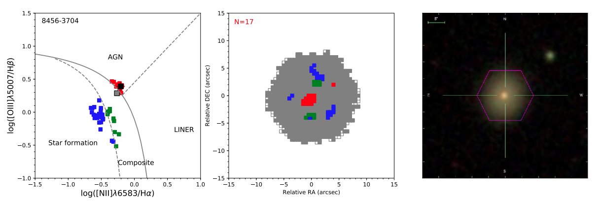
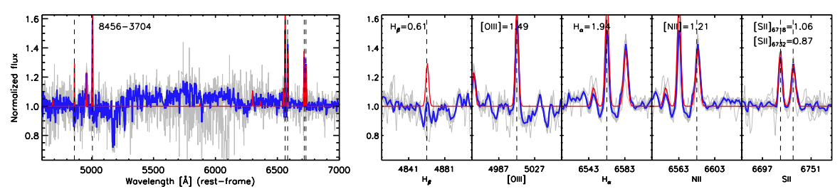
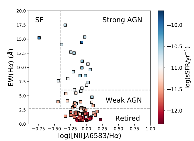
AGNs in this sample are identified in the optical part of the spectrum. This is typically done using the BPT diagnostic, where two optical emission line ratios are compared to distinguish between AGNs and star-formation as the primary source of ionisation. Due to the high redshift of the AGNs in this sample, however, some of the emission lines used in the BPT diagram do not appear in their spectra, rendering one of these ratios unusable. Instead, the authors turn to the mass–excitation diagram, which is based on the BPT diagram but replaces the lost emission line ratio with stellar mass. Enhancement of the remaining BPT ratio, called the excitation axis, can be caused by lower metallicity, but this only occurs in lower-mass galaxies, as they typically host younger stars. Given these are fairly high mass galaxies, we know that their metallicity is higher, so any increase in the excitation axis is due to AGN activity. This means the authors can identify AGNs by looking for enhancement in the excitation axis within these relatively high mass galaxies. Alongside this, they also apply a spectral signal-to-noise threshold to make sure these excitation detections are real.

Do AGN Quench Star Formation?

Taking these criteria together, the authors find a sample of 64 AGNs in the PSB sample, leading to an AGN fraction of about 5%. Only five AGNs were found in the comparison sample, leading to an overall AGN fraction of 1.4%. This reveals that AGNs are more likely to be found in PSBs than in a sample of regular galaxies of similar mass and redshift.

AGN fraction

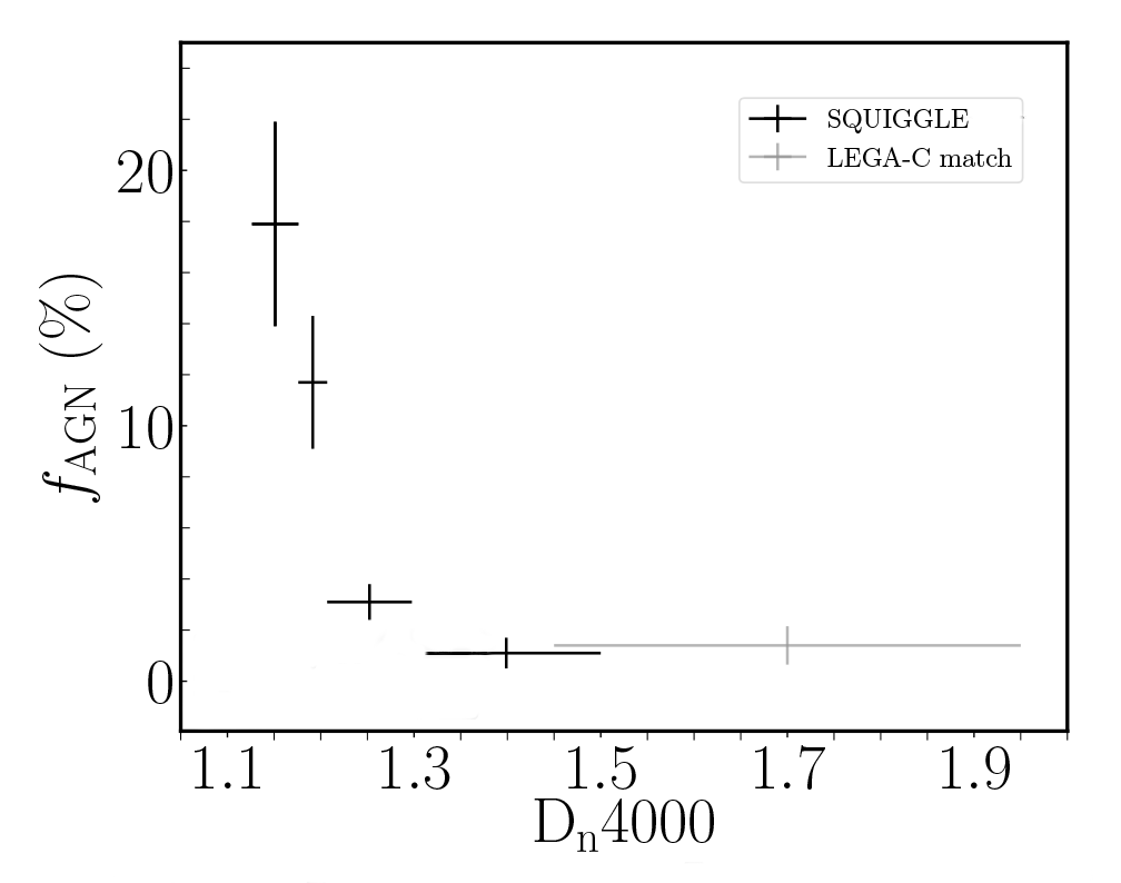
Figure 2: Comparing the AGN fraction as a function of galaxy age for the PSBs (taken from SQuIGGLE) and the normal galaxy sample (taken from LEGA-C). Dn4000 (4,000-angstrom break) describes the age of the galaxy, with a higher Dn4000 corresponding to an older galaxy. [Adapted from Greene et al. 2020]

These results are broken down further to identify how trends may vary with host galaxy properties. Most interestingly, they look at how AGN fraction varies with stellar age, measured using a quantity called the 4,000-angstrom break (Dn4000). It gives us an indication of the relative contributions made to a galaxy’s spectrum by the shorter-lived, blue stars and their longer-lived red counterparts. Once quenching has occurred, Dn4000 increases as the short-lived, blue stars start to die and cannot be replaced, leaving behind only longer wavelength emission from red stars. Figure 2 shows the results of this breakdown of AGN fraction with galaxy age.  It clearly shows that younger PSBs have an extremely enhanced AGN fraction compared to older ones: AGNs are ten times more likely to appear in the youngest PSBs!

AGN fractions appear to peak around the time of the quenching event where AGN-driven winds could force gas out of the host galaxy. In doing this, the AGN also removes sources of future fuel, causing the large drop in AGN fraction as the galaxies get older. Such a strong correlation between AGN fraction and the galaxy’s age suggests AGN activity could play a role in quenching galaxies. Whilst this correlation is compelling, it isn’t definitive. This makes the follow-up work being done by the authors all the more important: they are searching these AGNs for signs of outflows, which, if found, would suggest that star formation really is quenched by AGN-driven winds.

About the author, Keir Birchall:

Keir is a PhD student studying methods to identify AGN in various populations of galaxies to see what affects their incidence. When not doing science, he can be found behind the lens of a film camera or listening to the strangest music possible.

millisecond pulsar

Editor’s note: Astrobites is a graduate-student-run organization that digests astrophysical literature for undergraduate students. As part of the partnership between the AAS and astrobites, we occasionally repost astrobites content here at AAS Nova. We hope you enjoy this post from astrobites; the original can be viewed at astrobites.org.

Title: Gravitational-wave constraints on the equatorial ellipticity of millisecond pulsars
Authors: The LIGO Scientific Collaboration, the Virgo Collaboration
First Author’s Institution: Northwestern University
Status: Submitted to ApJ

Neutron stars represent one of matter’s weirdest manifestations. They have a mass of a little more than that of the Sun packed into a space the size of a big city — and getting to know their size, shape, and structure can unlock the most fundamental questions in atomic physics. What makes up a neutron star? Are they rigid or squishy? Are they perfectly spherical? If they have deformities, what is the tallest “mountain” they can support?

The first direct detection of gravitational waves by LIGO in 2015 gave us one of the best tools for studying neutron stars. Gravitational waves are radiated whenever matter moves in an asymmetric manner, which changes its quadrupole moment with time. For us to be able to detect these waves, they need to emanate from the asymmetric motion of extremely massive and dense matter. The first detection of gravitational waves was radiation from a pair of black holes spiraling into one another. Since then, most of the gravitational wave events detected by LIGO–Virgo have similarly been black hole binaries.

neutron star merger

Artist’s impression of the collision and merger of two neutron stars. [NSF/LIGO/Sonoma State University/A. Simonnet]

However, one might argue that neutron stars are much more diverse and interesting gravitational wave sources. The first confirmation of the existence of these waves was provided by the Hulse–Taylor binary: a system featuring a pulsar (a rapidly rotating neutron star giving off radio pulses) orbiting another neutron star. This week, we just passed the third anniversary of GW170817, an event where for the first time, LIGO and Virgo “heard” two neutron stars colliding. The collision resulted in a kilonova explosion that was observed using electromagnetic telescopes.

Neutron stars can exist in pairs and do the tango like the binaries mentioned above, but the cool thing is that they can also radiate gravitational waves while being single!

Any physical deformation, like a “mountain” on the neutron star crust, will give rise to a large quadrupole moment since neutron stars rotate extremely fast. The particular kind of neutron stars studied here are called millisecond pulsars: entire stars that complete one rotation within a few tens of milliseconds, much less than the blink of an eye. Even if the pulsar were perfectly spherical on the outside, it may have internal deformities in its core — a possibility that very little is known about. Or, it may be slightly elliptical in shape and wobble asymmetrically as it spins, which can also give rise to gravitational wave radiation.

All of the above mechanisms of lone neutron star gravitational waves have a tantalizing characteristic: their frequency is almost entirely constant. This is because it is determined by the frequency of rotation of the neutron star. These gravitational waves are thus known as continuous waves, distinguishing them from the transient, chirping waves produced by colliding binaries.

The search for continuous waves from pulsars is promising because data analysts know which frequencies to dig out from the data for the pulsars that astronomers have already seen through radio telescopes. This enables targeted searches for known millisecond pulsars in LIGO and Virgo data (Figure 1).

GW frequencies of known pulsars

Figure 1: The gravitational wave frequencies (dashed vertical lines) of known pulsars used in this search, compared with the power spectral density (PSD), also known as the “noise bucket of sensitivity” of the LIGO and Virgo gravitational wave observatories. The spikes in the PSD correspond to known continuous noise sources, such as the 60-Hz power line in the US. Can you see why it is such a nuisance for the Crab pulsar? [LIGO–Virgo Collaboration 2020]

LIGO–Virgo’s third observing run did not detect continuous waves from any pulsar directly. The downside of continuous wave searches is that the expected strength of these gravitational wave signals is far less than those from compact binary mergers. Assuming that continuous waves are constant in frequency, only long stretches of data spanning several years can build enough signal above the noise threshold. However, even a non-detection can tell us a lot about what the structure of the pulsar is (or more importantly, isn’t!)

It isn’t quite true that rotation speeds of pulsars are absolutely constant. Indeed, if an elliptical, wobbly pulsar radiates gravitational waves, it would invariably lose energy and slow down (called spin-down). Other factors, like magnetic fields or internal dynamics, can dominate this slowing down process as well. Pulsar spin-down has already been measured, but it takes place over very long timescales, effectively ensuring that pulsar frequency is constant over the period of a LIGO–Virgo observing run.

Knowing the spin-down rate helps us probe an interesting aspect of pulsars. Assuming that a pulsar slows down entirely due to radiation of gravitational waves and no other processes, conservation of energy equates the spin-down to the expected strength of gravitational waves detected. The energy of these gravitational waves is related to the degree of deformation or ellipticity of the pulsar. The observed spin-down limit thereby constrains the degree of asymmetry of the neutron star mass distribution as it rotates.

pulsar ellipticity

Figure 2: Constraints on the mass quadrupole moment Q22 and ellipticity for one of the pulsars in the study. The area under the curve between two values of quadrupole moment is the probability that the true value lies within that range; smaller values imply increasingly perfect spheres. The black vertical line represents the spin-down limit for the pulsar, and the colored vertical lines correspond to 95% confidence that the ellipticity is below a certain value. When the upper limit measurements (colored vertical lines) of the quadrupole moment (or ellipticity) lie to the left of the black lines, the spin-down limit has been surpassed. [Adapted from LIGO–Virgo Collaboration 2020; reference here]

For the very first time, LIGO and Virgo achieved a level of sensitivity that enabled them to detect possible signals from the pulsar J0711–6830 weaker than its known spin-down limit (Figure 2). That means the authors could constrain its ellipticity or limit the size of its mountains to a greater extent than previous observations. As a result of not detecting any gravitational waves, we now know that this pulsar is less deformed from a perfect sphere than the width of a human hair!

Before Galileo pointed his telescope towards it, most scientists believed that the Moon was a perfect sphere. It is fascinating today to be able to correctly identify perfect spheres over a hundred times smaller than the Moon, situated over 300 light years away from us.

About the author, Sumeet Kulkarni:

I’m a third-year PhD candidate at the University of Mississippi. My research revolves around various aspects of gravitational wave astrophysics as well as noise characterization of the LIGO detectors. It involves a lot of coding, and I like to keep tapping my fingers on a keyboard even in my spare time, creating tunes instead of bugs. I run a science cafe featuring monthly public talks for the local community here in Oxford, MS, and I also love writing popular science articles. My other interests include reading, cooking, cats and coffee.

Orion Nebula

Editor’s note: Astrobites is a graduate-student-run organization that digests astrophysical literature for undergraduate students. As part of the partnership between the AAS and astrobites, we occasionally repost astrobites content here at AAS Nova. We hope you enjoy this post from astrobites; the original can be viewed at astrobites.org.

Title: Winds in Star Clusters Drive Kolmogorov Turbulence
Authors: Monica Gallegos-Garcia, Blakesley Burkhart, Anna Rosen, Jill P. Naiman, and Enrico Ramirez-Ruiz
First Author’s Institution: Northwestern University
Status: Published in ApJL

Turbulence, or chaotic changes in the pressure and velocity of a fluid, is one of the great mysteries of classical physics. Much of the gas in galaxies is known to be turbulent, but the mechanisms that developed and maintain this turbulence remain areas of active research. While we still don’t know all the details of the physics behind turbulence, a lot of time and effort has gone into identifying statistics that can tell us whether gas is turbulent or not. In other words, we know what turbulence looks like even if we don’t know all the details of how it works (see this Youtube video for a great introduction to turbulence and the power spectrum, a statistic used in today’s paper). Today’s weather forecast calls for strong winds blowing in from the arXiv as we explore a new paper studying how stellar winds from star clusters can drive such turbulence.

Stellar winds, particularly those from massive stars like O or B types, blow bubbles in the surrounding cold gas by pushing it outwards and leaving a cavity behind. These are analogous to the bubbles we see on Earth that are created by air pushing into some other medium. In the case of a stellar-wind bubble, the “air” is hot stellar wind material. When massive stars are found in a star cluster, their bubbles tend to overlap and form a “superbubble”. One incredible example of this is the Orion Nebula Cluster (see the cover image above). The authors of today’s paper run simulations that roughly mimic the stellar profile of the Orion Nebula Cluster, and they too find the creation of large superbubble.

In these simulations, the most massive stars expel high-velocity, hot gas that fills the superbubble and pushes it outwards into cooler gas. This expansion produces a thick shell at an intermediate temperature (Figure 1). Because this shell is more dense than the central hot gas, it is able to cool faster and remain much cooler than the superbubble interior. As the simulations progress, turbulent instabilities appear in the hot gas inside the shell.

expanding superbubble

Figure 1: Plots of the expanding superbubble created by winds from massive stars. The most massive stars are shown in blue and purple, and these are the ones that primarily contribute to the bubble expansion. Top: Density slice, with high-density material shown in darker colors and low-density material shown in lighter colors. Bottom: Temperature slice, with hotter material shown in lighter colors and cooler material shown in darker colors. Time is shown in kyr (1 kyr = 1,000 years). [Gallegos-Garcia et al. 2020]

One interesting result of these simulations is the diversity in speeds at which the gas is traveling. Figure 2 shows plots of the Mach number of the gas, a measure of how quickly gas is traveling relative to the sound speed of the gas. This is the same Mach number that is used to discuss very fast cars or planes — anything traveling at a speed greater than Mach one will result in a supersonic shock. In this case, the shell of the bubble is traveling at a Mach number greater than one as a supersonic shock that pushes into the surrounding material. However, Figure 2 also demonstrates that interior gas is almost entirely subsonic and subject to strong fluctuations in velocity throughout the bubble. In other words, even though the stellar winds drive a supersonic shock, they produce subsonic turbulence inside the bubble.

velocities in superbubble

Figure 2: Plots of gas velocities in the expanding superbubble. The mass of the stars is denoted the same way as before. The Mach number is shown as a logarithm, meaning that negative numbers correspond to a Mach number less than one, zero corresponds to a Mach number of one, and positive numbers correspond to a Mach number greater than one. Time is shown in kyr (1 kyr = 1,000 years). [Gallegos-Garcia et al. 2020]

In order to ensure that the hot gas inside the bubble is actually turbulent, the authors choose a statistic known as the power spectrum, which allows them to see how energy moves from large scales in the simulation down to small scales. Figure 3 shows the power spectrum at different times in the simulation. The typical expected power spectrum for subsonic turbulence is a power law with a slope of –5/3 (known as Kolmogorov turbulence). The authors find that their simulation roughly approaches this as time evolves, indicating that stellar winds are in fact driving primarily subsonic turbulence.

velocity power spectrum

Figure 3: Density-weighted velocity power spectrum for different times in the simulation. The dashed line indicates the expectation for subsonic turbulence. The y-axis shows the power spectrum, and the x-axis denotes the wavenumber. See this video for an explanation of the power spectrum. [Gallegos-Garcia et al. 2020]

This is an exciting result that indicates star clusters may have a significant role to play in driving and maintaining turbulence in galaxies. Modeling turbulence is crucial to understanding many processes in galaxy evolution, such as star formation. Through simulations like these, astronomers can get a better idea of exactly why gas in galaxies behaves the way it does and how it can form new stars, solar systems, and even us.

About the author, Michael Foley:

I’m a graduate student studying Astrophysics at Harvard University. My research focuses on using simulations and observations to study stellar feedback — the effects of the light and matter ejected by stars into their surroundings. I’m interested in learning how these effects can influence further star and galaxy formation and evolution. Outside of research, I’m really passionate about education, music, and free food.

HD189733b

Editor’s note: Astrobites is a graduate-student-run organization that digests astrophysical literature for undergraduate students. As part of the partnership between the AAS and astrobites, we occasionally repost astrobites content here at AAS Nova. We hope you enjoy this post from astrobites; the original can be viewed at astrobites.org.

Title: Transit signatures of inhomogeneous clouds on hot Jupiters: Insights from microphysical cloud modelling
Authors: Diana Powell et al.
First Author’s Institution: University of California, Santa Cruz
Status: Published in ApJ

A Crash Course on Transmission Spectroscopy

Much of our knowledge about the atmospheric properties of exoplanets comes from transmission spectroscopy. An exoplanet’s apparent size (inferred from the amount of starlight it blocks out) varies with wavelength as molecules (plus atoms, ions, clouds, or hazes) in the upper layer of the exoplanet’s atmosphere absorb different wavelengths of the star’s light. Clouds are especially important, as they affect atmospheric spectra and inhibit our ability to learn about the fundamental atmospheric properties for the majority of exoplanets (one example of this is shown in Figure 1). Not only are atmospheric clouds ubiquitous in our solar system, but many exoplanets show strong evidence for clouds (for example, GJ 1214b and HD 209458b)!

transmission

Figure 1: a) Clouds block the transmission of starlight, producing a flat transmission spectrum with dampened/weakened features. b) A clear atmosphere (with no clouds) allows starlight to penetrate deeper into the atmosphere, where molecules such as water absorb light. The resulting transmission spectrum has absorption spectral features, which enable astronomers to infer the molecular composition of the atmosphere [Eliza Kempton]

Typical transmission spectra analysis methods, like atmospheric retrievals, assume a 1D atmosphere that only changes radially, because working with detailed 2D/3D models is computationally challenging. However, as you might have guessed, planets are 3D! The transmission spectra we collect in our telescopes are a combination of multiple spectra from different locations in the atmosphere. Atmospheric composition and temperature can vary in 3D, and the distribution of clouds on a planet can also be wildly inhomogeneous, i.e., non-uniform.

The Case of Hot Jupiters

A category of exoplanets called hot Jupiters (Jupiter-like gas giants orbiting very close to their host stars) are especially likely to have non-uniform cloud distributions. Because hot Jupiters are tidally locked, their daysides and nightsides have huge temperature contrasts. Cloud properties are highly sensitive to how the temperature of the atmosphere changes with height, longitude, and latitude (referred to as the atmosphere’s “local thermal structure”). So, we expect that a hot Jupiter will have clouds with diverse properties (for example, on Earth, water clouds form where it is cold enough for water to condense). In particular, models show that for many hot Jupiters, the thermal structure on the east limb is substantially hotter than the temperature on the west limb (see Figure 2). Since various gases condense to form clouds at different temperatures, this leads to clouds with very different properties forming on the east limb versus the west limb.

hot Jupiter atmosphere

Figure 2: A schematic of the atmospheric regions along the terminator of a hot Jupiter: the poles (green), east limb (red), and west limb (blue). This is the view of the dayside of the planet, the side always facing the star. The substellar point is the point on the dayside of the planet that is closest in distance to the star. [Powell et al. 2020]

We have evidence for non-uniform clouds through phase curve observations of hot Jupiters (and brown dwarfs), where we observe how the reflected starlight from the planet changes as the planet orbits its host star. However, various difficulties with obtaining phase curve measurements make this method of probing cloud cover difficult to generalize to the vast majority of exoplanets. One promising alternative is transmission spectroscopy. Today’s paper explores if transit measurements of hot Jupiters with the James Webb Space Telescope (JWST) can provide a strong signature of non-uniform clouds.

How Do Non-Uniform Clouds Affect the Transmission Spectrum of a Hot Jupiter?

In today’s article, the authors present transmission signatures of non-uniform cloud cover on hot Jupiters that should be observable using the JWST, scheduled for launch later next year. First, the authors try to understand how temperature structure and composition differences produce these non-uniform clouds, and consequently, the observed transmission spectrum of the planet.  We should also note that because hot Jupiters have very high equilibrium temperatures (~2,000 K), the clouds are composed of molecules that can condense at these temperatures, like silicates, aluminum, and titanium oxides (wild!).

The authors simulate cloud formation on various Jupiter-sized, tidally locked planets orbiting a solar-type star. The differences in cloud structure between the east and west limbs of these model hot Jupiters manifest as differences in the transmission spectra of their east and west limbs. An example transmission spectrum for a planet with equilibrium temperature of 2,000 K is shown in Figure 3 and discussed below:

  1. Firstly, the model transmission spectra are different on each limb of the planet, often by as much as ~1,000 ppm or parts per million.
  2. Secondly, the west limb spectrum appears very flat with subdued molecular features, because it’s much more cloudy.
  3. Thirdly, the overall absorption in the east limb is higher (larger transit depth values), especially at shorter wavelengths, because clouds form at much higher altitudes on the east limb where it is hotter. Thus the apparent radius of the planet at shorter wavelengths, where clouds are opaque, is much larger on the eastern limb than the western limb, creating a ~1,000 ppm difference in transit depth.
  4. Finally, it’s interesting to note that the east limb, despite forming fewer clouds, provides a more clear signature of the properties of the clouds (the aluminum + silicate bump at ~10–20 microns) present in the atmosphere.
model transmission spectra

Figure 3: Model transmission spectra (black lines) for a hot Jupiter with an equilibrium temperature of 2,000 K at the east and west limbs. The blue lines show the absorption contribution only from clouds (absorption from gases is excluded). The cloud-free transmission spectrum at the east limb is shown in gray. At the west limb, clouds dominate the spectra at all wavelengths. At the east limb, clouds contribute to muted transmission features at short wavelengths and a sloped optical spectrum. There is a relatively clear window at ~5–9 microns and enhanced silicate and aluminum cloud opacity from 10–20 microns. [Powell et al. 2020]

Strategies for Observing Cloud Non-Uniformity with JWST

The authors explore whether JWST will be capable of detecting non-uniform clouds on exoplanets through transit curve observations.

planet model

Figure 4: Top: Diagram of the model used to simulate a planet at 2,100 K, where the additional atmosphere height is highlighted in green and has been inflated by a factor of 5 for clarity. Middle: The light curves calculated for these planet geometries. Bottom: The difference between the two light curves. The presence of an asymmetric atmosphere leads to a characteristic signature. [Powell et al. 2020]

They first investigate how the transit curve of a non-uniform exoplanet atmosphere compares with one with a uniform atmosphere. They find that the transit lightcurves show characteristic differences (Figure 4), which also vary with wavelength. Importantly, the magnitude of these differences are within the detection capability of JWST.

Next, the authors investigate if cloud properties (uniform vs. nonuniform) can be recovered from simulated JWST transit curves (fake JWST data) in two wavelength channels (at 1 and 6 µm). They simulate lightcurves for the two wavelength regions, using a JWST simulator, and then attempt to fit these lightcurves and recover the parameters used to initially generate the model. As expected, they find that a model with a non-uniform atmosphere, especially when clouds are included, does a much better job fitting the synthetic data as compared to a model with a uniform atmosphere.

To Sum it Up…

This work provides a detailed insight into how the differences of cloud distribution on the east and west limbs of a particular kind of exoplanet — hot Jupiters — are reflected in its transmission spectrum and transit light curves. The authors provide techniques which should enable us to uncover cloud inhomogeneities (or non-uniformities) with the much awaited JWST, as a complementary method to the more common phase curve studies of exoplanet atmospheres. This work is a key step forward as the exoplanet community moves towards understanding exoplanet atmospheres as inherently complex 3D entities.

About the author, Ishan Mishra:

I am an astronomy PhD candidate at Cornell University. As a planetary scientist, I am interested in analysis/retrieval techniques of the abundant spectroscopic data in the field. Currently, I mostly work on analyzing new (and old) reflectance data of Europa, with the goal of building a comprehensive picture of its surface composition. I also delve into exoplanet transmission data from time to time, where my interests lie in the new and exciting retrieval techniques which exoplanet science is pioneering. Outside of science, I am interested in listening to and playing music, tennis, (the real) football, hiking, museums and historical/archeological tours.

Antennae galaxies

Editor’s note: Astrobites is a graduate-student-run organization that digests astrophysical literature for undergraduate students. As part of the partnership between the AAS and astrobites, we occasionally repost astrobites content here at AAS Nova. We hope you enjoy this post from astrobites; the original can be viewed at astrobites.org.

Title: Stellar and Molecular Gas Rotation in a Recently Quenched Massive Galaxy at z ∼ 0.7
Authors: Qiana Hunt et al.
First Author’s Institution: Princeton University
Status: Published in ApJL

We know that as they age, galaxies transition from blue, star-forming disks to red, quiescent ellipticals, but the stages of evolution and the process of stopping star formation (often called quenching) are still mysterious. One clue to answering these questions may be post-starburst galaxies, or galaxies that recently experienced a period of intense star formation and are now calm and quiet. The authors of today’s paper explore the properties of the stars and gas in a post-starburst galaxy to explain what mechanisms may have stopped the star formation.

The Starting Line-Up

Post-starburst galaxies are generally full of A-type stars. This means their period of star formation must have stopped a few billion years ago, within the lifetime of main sequence A-type stars. The quenching mechanism for star formation (basically, whatever turns it off) is thought to leave a signature, but that signature deteriorates over time, so it is essential to look at galaxies right after their star formation stops.

SDSS J0912+1523 is a recent and unusual post-starburst galaxy. Its molecular gas mass is around 30% of the stellar mass, much higher than other similar galaxies, which makes it an interesting target. Figure 1 shows the galaxy. On the left is the flux map, which shows the brightest portions of the galaxy in green. There are two main peaks at the center of the galaxy, which might indicate that the galaxy has two cores. On the right is the galaxy separated into spatial bins, with different shaded grey regions representing different bins that will be used later. The flux contours are overlaid to again show the brightest portion, and the rightmost squiggly line shows the combination of flux and noise across the galaxy.

SDSS J0912+1523

Figure 1: Left: The flux map of SDSS J0912+1523, a post-starburst galaxy. Green represents higher flux, while dark blue represents lower flux. The two central peaks in the flux represent two possible cores. Right: The galaxy sectioned into bins (differing shades of grey) with flux contours overlaid in the same colors as in the left plot. The purple line on the right side shows the combination of flux and noise across the galaxy. [Hunt et al. 2020]

Moving As A Team

The authors of today’s paper used spectroscopy from Gemini Observatory to look at the properties of stars in the galaxy. They looked for oxygen emission lines that generally indicate star formation and found none, which is to be expected for a quenched galaxy. The authors did, however, find lots of hydrogen Balmer absorption lines, because A-type stars have very strong Balmer lines in their spectra. The depth of those lines can actually be used as a proxy for stellar age. The deeper the absorption line, the more recent the star formation episode.

To quantify how deep the Balmer lines were in each spectra, the authors used an equivalent width. When an absorption line dips below the continuum, there is a certain area between the curve and the continuum. The equivalent width is how much of the continuum (in this case in Angstroms) it would take to make a rectangle with that same area underneath. The equivalent widths in the center of the galaxy can be seen in the top row of Figure 2. On the left, the figure shows the values for the equivalent width with position in the galaxy, while on the right it shows the equivalent width with distance from the center of the galaxy. The equivalent width doesn’t change much within the inner part of the galaxy, which means that all the stars are probably from a common population that formed at the same time.

The spectra were also used to find velocities and velocity dispersions, as shown in the second and third rows of Figure 2. The velocity map and trend with distance from the center of the galaxy shows that the galaxy is clearly rotating, as one side is moving away from us and one side is moving towards us. The consistency in the velocity dispersion indicates that the two cores (the two peaks in intensity that we saw above) are the same galaxy rotating as a single object. The authors suggest the two cores might be remnants of a galaxy merger or a single core with a lane of dust obscuring part of it.

galaxy properties

Figure 2: Top row: The first column shows the equivalent width of the hydrogen Balmer absorption line for bins in the center region of the galaxy. Larger values correspond to more recent star formation. The second column shows the equivalent width with distance from the center of the galaxy, color-coded by signal-to-noise. Middle row: Velocity within binned regions of the galaxy and velocity with distance from the center. The galaxy is clearly rotating, with one side blueshifted and the other redshifted. Bottom row: The same as seen in the other rows, but for velocity dispersion. [Hunt et al. 2020]

Subbing In A New Player

The authors of today’s paper also compared their findings to ALMA data that shows the galaxy’s molecular gas content. Figure 3 shows the comparison of stellar (left) to molecular gas (right) velocities. The stellar velocities very closely resemble the molecular gas velocity, so the stars and gas are likely rotating together.

velocity map

Figure 3. The velocity map for stellar velocity from this paper (the same as in Figure 2) compared to cold molecular gas in the galaxy (from ALMA data). The similarity indicates that the stars and the gas are rotating together. [Hunt et al. 2020]

Hydrating A Galaxy

So what does this information tell us about the star-formation quenching mechanism? There are a lot of ideas about what might stop star formation. Galaxy mergers might heat up gas and prevent it from collapsing into stars. Gas might fall to the center of galaxies, creating star formation there but leaving an empty outer part of the galaxy, or it might get ejected altogether in an outflow. Each of these scenarios is expected to result in a certain amount of velocity dispersion and cold molecular gas. And this galaxy? Because of its large molecular gas content and stable velocity dispersion, it doesn’t fit well with any of these scenarios. Today’s authors suggest that something else might be at play — a type of quenching where the disk of a galaxy stabilizes itself from collapse, the very thing that causes star formation.

This target is a very interesting example of the transition from star-forming to quiescent galaxies. Continuing to study subjects like it will allow astronomers to determine how galaxies become red and dead.

About the author, Ashley Piccone:

I am a second year PhD student at the University of Wyoming, where I use polarimetry and spectroscopy to study the magnetic field and dust around bowshock nebulae. I love science communication and finding new ways to introduce people to astronomy and physics. In addition to stargazing at the clear Wyoming skies, I also enjoy backpacking, hiking, running and skiing.

Fornax dwarf galaxy

Editor’s note: Astrobites is a graduate-student-run organization that digests astrophysical literature for undergraduate students. As part of the partnership between the AAS and astrobites, we occasionally repost astrobites content here at AAS Nova. We hope you enjoy this post from astrobites; the original can be viewed at astrobites.org.

Title: Populating the Low-mass End of the MBH–Mσ∗ Relation
Authors: Vivienne Baldassare et al.
First Author’s Institution: Yale University
Status: Published in ApJL

Dwarf galaxies are believed by some to be time capsules, but instead of old records, they are thought to preserve the seeds of black holes formed in the early universe. This is because most dwarf galaxies detected in the nearby universe don’t show signs of interacting with their galactic neighbours, leaving these relatively low-mass collections of gas, dust, and stars to evolve in isolation. Without contamination from other galaxies, astronomers can treat these dwarf galaxies as pristine pockets of the universe’s past. So by analysing the distribution and masses of the black holes in these dwarf galaxies, astronomers can hope to shed some light on how they formed.

pop iii stars

Artist’s impression of the first stars in the universe. [NASA/WMAP Science Team]

Two formation mechanisms dominate discussion: either black holes formed from the collapse of early generations of stars, known as Pop III stars, or they formed from the direct collapse of gas and dust. If the former mechanism dominates then we would expect to find large numbers of low-mass black holes, while the latter mechanism is predicted to produce a much smaller number of higher-mass seeds. Unfortunately, dwarf galaxies are much fainter than their higher-mass counterparts, so they are difficult to detect. The often invisible black holes within provide an even greater challenge.

An easier way to detect these black holes is to wait for them to accrete material and emit huge amounts of radiation, turning them into a source known as an active galactic nucleus (AGN). Over the past decade, there has been a huge increase in the number of AGNs detected in dwarf galaxies. Today’s authors aim to place some of these AGNs on a well-known mass & velocity dispersion relation to try and gain insight into how black holes may have formed in the early universe.

Finding the AGNs

Active Galactic Nucleus

Artist’s impression of the thick shroud of dust hiding a galaxy’s active nucleus. [NASA/SOFIA/Lynette Cook]

The previous work that the authors draw on takes galaxies from the NASA–Sloan Atlas and identifies any AGNs therein using the BPT diagnostic (named after its creators Baldwin, Phillips & Terlevich). This technique compares the ratio of two optical emission line pairs to determine whether the host galaxy’s spectrum is dominated by AGN processes, star-formation processes, or is a composite of both. In addition, the objects were also required to have broad-line Hα detections, as these are used to calculate the virial mass of the black hole. Aspects of the Hα emission describe the behaviour of the broad line region (BLR), the highly ionised inner region of a galaxy hosting an AGN. Measuring the luminosity and full-width half-maximum of the Hα line can be used to infer the BLR’s radius and velocity of the material therein. With this data, the authors can calculate the black hole mass. From these criteria, the authors identified eight objects that have broad-line Hα emission and are classified as either AGN or composite by the BPT diagnostic.

While velocity dispersion can be measured from the Hα line, it is important that this quantity is independent from the black hole mass. So, for each of these AGNs the authors used the Keck II Echellette Spectrographer to measure the Mg Ib triplet and, where possible, the Ca II triplet. Where both lines were available, the overall velocity dispersion was calculated using the mean of both measurements. Unfortunately, some galaxies occupy redshifts that cause significant contamination at the Ca II wavelengths, so when the Ca velocity dispersion wasn’t available the Mg Ib value was used.

How Low Can You Coevolve?

Today’s paper has doubled the number of black holes in dwarf galaxies plotted on the mass & velocity dispersion relation. Figure 1 shows the results of these measurements and compares them to numerous others across the mass spectrum. It is quite striking that all the AGNs identified in the sample are consistent with the plotted relations. Finding low-mass black holes that lie on these relations can help extend the mass range over which we believe black holes and their host galaxies directly interact. Today’s results show further evidence suggesting that black holes in dwarf galaxies interact with their hosts in similar ways. With this knowledge, astronomers can better understand how black holes across the mass spectrum grow and interact with their galaxies.

m-sigma plot

Figure 1: Black hole mass vs. velocity dispersion for galaxies across the mass spectrum. The two lines represent fits to different galaxy samples: the solid line is fit to galaxies with bulges, the dashed line is fit to broad-line AGNs. [Baldassare et al. 2020]

While this is a valuable result on its own, today’s authors were also interested in what the black hole masses can tell us about how they formed in the early universe. If stellar collapse dominated early black-hole formation, then the authors would have expected the black holes to be under-massive and trace out a steeper slope. On the other hand, if direct collapse dominated, then we would expect the black holes to be over-massive and trace out a flatter curve. Unfortunately, the fact that these masses are all consistent with the plotted relationships does not provide a definitive answer as to which mechanism is more likely.

However, the authors do try to draw some conclusions from the single black hole (blue, square data point) at the bottom of figure 1 and fact that their black holes were all found because they were AGNs. As was previously mentioned, AGNs are black holes accreting material at a high rate, which not only causes the black holes to emit radiation but also increases their mass. Because of this accretion, the authors believe their detections might be black holes that are more massive relative to the rest of the dwarf-galaxy-hosted population of black holes. The extremely low-mass black hole at the bottom of figure 1, which is not an AGN, may be an example representative of this broader dwarf-galaxy black hole population, according to the authors. If this assumption is correct, it would point toward stellar collapse as the favoured mechanism of formation in the early universe. While this is an interesting argument, it is still somewhat speculative. Before we can make strong conclusions about how black holes formed in the early universe, numerous more measurements will need to be made to determine whether such extremely low black hole masses are the exception or the rule.

About the author, Keir Birchall:

Keir is a PhD student studying methods to identify AGN in various populations of galaxies to see what affects their incidence. When not doing science, he can be found behind the lens of a film camera or listening to the strangest music possible.

dwarf star planet

Editor’s note: Astrobites is a graduate-student-run organization that digests astrophysical literature for undergraduate students. As part of the partnership between the AAS and astrobites, we occasionally repost astrobites content here at AAS Nova. We hope you enjoy this post from astrobites; the original can be viewed at astrobites.org.

Title: An astrometric planetary companion candidate to the M9 Dwarf TVLM 513−46546
Authors: Salvador Curiel et al.
First Author’s Institution: National Autonomous University of Mexico (UNAM)
Status: Published in AJ

Finding Planets

Kepler planets

This artist’s illustration depicts multiple examples of planetary systems we’ve discovered. [NASA/W. Stenzel]

Since the first detections of planets outside of our solar system in the 1990s (for a review see this link), the exoplanet field has quickly grown. Initially, exoplanet detections were dominated by searches for Doppler shifts in the spectra of bright stars caused by the gravitational pull of one of more planets (known as the radial velocity method). In the last decade however, space-based satellites such as Kepler and TESS have shifted the focus to the transit method, or searching for small dips in the light received from stars as planets pass in front of them.

However, these are not the only methods we can use to find planets. Astronomers have also made use of the light-bending power of gravity (known as microlensing) to find planets, which is a major science goal of the upcoming Nancy Grace Roman Space Telescope. Sometimes, it is even possible to directly image a planet if the light of the host star can be blocked. Combined, these various methods have allowed us to find more than 4,000 exoplanets orbiting stars other than our Sun.

Wobbly Stars

There is one exoplanet detection method that we haven’t discussed yet, known as the astrometric method. This method essentially looks at the position of a star over a period of time and tracks deviations from the expected position. Discovering a planet this way requires excellent precision though. Fortunately, the Gaia satellite is capable of making such a measurement, and it is expected that by the end of the mission that we will find many new planets through this method (for more details see this bite). With that said, there is only one currently claimed discovery of an exoplanet through astrometry. Today’s paper increases that count to two!

M dwarfs, stars cooler than our Sun, are one of the major targets for exoplanet searches due to their large numbers in our galaxy and the fact that habitable exoplanets around M-dwarfs are some of the best candidates for atmospheric characterization. In this paper, the authors look at the M9 dwarf TVLM 513 (with a mass of 0.06–0.08 solar mass), which had been a target for earlier studies in the radio using very-long-baseline interferometry (VLBI). The authors combine archival VLBI data with new observations to produce the stellar motions shown in Figure 1.

VLBI data

Figure 1: Parallax fits to the VLBI data. The left panels are the new data and the right panels are the combined archival+new data. The upper panels show the fit using only the proper motions and the parallax of TVLM 513. The middle panels show the residuals in right ascension and the bottom panels show the residuals in declination. The temporal trend in the residuals suggests the presence of a companion. [Curiel et al. 2020]

In Figure 1, there are two clear types of motion of TVLM 513. The first is the general motion from the upper left to the bottom right, caused by the proper motion of the star on the sky. The second is a back-and-forth motion known as parallax, which is caused by the Earth’s orbit around the Sun. At first glance, the observed positions of the star appear to follow these two general trends well, but there are small deviations from this path that are shown in the bottom two panels of Figure 1. This tells the authors that there is something tugging on their star, which in this case turns out to be a planet!

From their fits to the observed astrometric signal, the authors find a companion at a period of P = 221 ± 5 days, with a circular orbit, a mass of m = 0.35−0.42 Jupiter masses, a semi-major axis of a = 0.28−0.31 au, and an inclination angle of i = 71−88° (where 0° is face-on and 90° is edge-on). This discovery of the planet TVLM 513b is only the second astrometric discovery of a planet to date. It is also the first planet detection to use radio astrometry.

TVLM 513b in Context

With a new (Saturn-like) planet in hand, the authors turn towards the wealth of exoplanet observations to understand how their exciting new discovery fits in with the broader picture. To do this, the authors create Figure 2, which compares the host stellar mass to the planetary mass and the semi-major axis of the planet’s orbit. In comparison to most known planets, TVLM 513b orbits a much lower-mass star. While the TESS mission will begin to add new planets discovered around other low-mass stars, astrometry will continue to be an effective method for finding planets around such stars. TVLM 513b itself is somewhat moderate in terms of its mass and semi-major axis compared to other planets. Combined, this system lies in a relatively unexplored region of parameter space. Most other planets in this region were found using microlensing, which unfortunately does not allow for detailed follow-up observations.

planet comparison

Figure 2: Comparison of fundamental properties of planets and their orbits as a function of discovery method. Left: Comparison of stellar mass and planetary mass. Right: Comparison of stellar mass and semi-major axis of the planet. In both panels, green points are radial velocity, blue are transit, pink are imaging, red are microlensing, and yellow are astrometry discoveries. The black stars are the location of TVLM 513b using the upper and lower mass limits for the host star. [Curiel et al. 2020]

The authors also note that the parameters of this planet are somewhat unexpected given commonly accepted theories of planet formation. The two main theories for the creation of giant planets are core accretion and disk instability. For core accretion, the masses of planets should scale with their host star, so a massive planet around such a low mass star is unexpected. While disk instability can create massive planets around low mass stars, both models predict massive planets to occur at least a few au from the central star, whereas TVLM 513b has a semi-major axis of ~0.3 au. The authors note that planet could have formed farther out and migrated in — but how and why did it stop at 0.3 au?

In brief, the authors of today’s paper have found a new planet through radio astrometry. But their discovery amounts to more than that. It is further proof that astrometry can not only find planets, but prompt new questions that will continue to drive the exoplanet field forward. This planet, combined with the many that continued TESS and Gaia observations and future missions will yield, will answer outstanding questions and pose even harder ones as we try to understand the origins of planetary systems both far away and closer to home.

About the author, Jason Hinkle:

I am a graduate student at the University of Hawaii, Institute for Astronomy. My current research is on multi-wavelength photometric and spectroscopic follow-up of tidal disruption events. My research interests also include a number of topics related to AGN, including outflows, X-ray spectroscopy, and multi-wavelength variability. In addition to my love for astronomy, I enjoy hiking, sports, and musicals.

disk snowline

Editor’s note: Astrobites is a graduate-student-run organization that digests astrophysical literature for undergraduate students. As part of the partnership between the AAS and astrobites, we occasionally repost astrobites content here at AAS Nova. We hope you enjoy this post from astrobites; the original can be viewed at astrobites.org.

Title: An ALMA Survey of H2CO in Protoplanetary Disks
Authors: Jamila Pegues, Karin Oberg, J. Bergner et al.
First Author’s Institution: Center for Astrophysics | Harvard & Smithsonian
Status: Published in ApJ

Person. Woman. Man. Camera. TV. What do all of these have in common? They are complex organisms or objects which are made of organic molecules. If we want to understand the origins of such earthly things, we need to understand how and where they form within protoplanetary disks. H2CO, or formaldehyde, is one of the most abundant organic molecules in the universe, and it can serve as a precursor to more complex organic molecules. Observing the location at which H2CO resides within a disk will provide insight into its formation, and thus the protoplanetary disk’s ability to form more complex molecules. Today’s paper surveys 15 protoplanetary disks looking at multiple H2CO lines. The authors seek to uncover the temperature, density, and origin of H2CO, which will inform our knowledge of chemistry within disks.

How Do You Form Molecules in Space?

There are two main formation pathways to form molecules within protoplanetary disks. You can form molecules in the gas via gas-phase chemistry, or you can form molecules on ice grains via ice–grain chemistry. Astronomers have seen that it is possible to create H2CO in both the gas phase and on grains, however we won’t know what the most common formation mechanism is within disks until we observe them. If H2CO is predominantly formed in the gas phase, we would expect to see a significant amount of H2CO near the center of a disk. This is because the inner few AU is where the gas is most dense, thus there is a higher likelihood of collisions between molecules that can form H2CO. If, on the other hand, ice–grain chemistry is the most common way to form H2CO, then we would expect to see a ring-like structure when observing the H2CO within a disk. This is because molecules “freeze out” onto grains at a certain temperature. To form H2CO on a dust grain, we need the molecule CO (carbon monoxide) to be chillin’ out on the dust grains. Chuck some hydrogen at it until it becomes H2CO, then it can be released off the grain for us to observe. So! We need CO to be not in the gas, but instead on the grains available for hydrogen to be thrown at them. That will only happen when the environment is so cold that CO begins to “freeze” onto dust grains, which only occurs pretty far away from the central star. That freeze-out location is called a snowline. Thus, if CO needs to be stuck onto ice grains to form H2CO, then we’d only see H2CO near the CO snowline, which will look like a ring around the star.

H2CO location in disk

Figure 1: A cartoon representation of the location of H2CO if its primary formation mechanism was gas-phase chemistry (left) or ice-grain chemistry (right). [Astrobites]

¿Por qué no los dos?

After observing H2CO towards 15 disks, what did these authors find? They found that eight out of 15 observed disks had H2CO that peaked in the center, three had little “dips” (so there was not a super significant amount of H2CO), and two had no H2CO flux in the center. At the same time, they found that six out of 15 of their disks had ring-like structures, or plateaus of flux continuing from the center of the disk.

emission maps of four disks

Figure 2: The emission maps of four different disks with multiple detections of transitions of H2CO. J1604-2130 (second from the top) is a great example of a disk that had missing H2CO flux in the center, plus ring-like structure, which suggests H2CO forms on ice grains in this disk. DM Tau (top) shows H2CO flux in the center of the disk, however it continues to extend quite far out, suggesting both gas-phase chemistry and ice–grain chemistry is taking place. [Pegues et al. 2020]

The authors determine that the observed structures are likely due to the chemistry that forms H2CO — as opposed to pesky dust getting in the way of seeing the real structure, or old H2CO that might have stuck around from a time before the formation of the protoplanetary disk. From this, they conclude that BOTH gas-phase and ice–grain chemistry are actively forming H2CO within disks.

A Gift That Keeps On Giving

Not only do these observations of H2CO tell us about the formation pathways of this organic molecule, but they also provide measurements of temperature and density within the disks. For disks with multiple line observations corresponding to different energetic transitions of H2CO, the authors can do some physics magic to pull out the excitation temperature and column densities of H2CO. With that information, they can then compare the densities of H2CO between different types of disks. They see a difference between the biggest and warmest disks (Herbig Ae disks) and the cooler smaller disks (T Tauri disks). The Herbig Ae disks tend to have less H2CO than the lower mass/cooler counterparts. This is consistent with other lower resolution observations of H2CO. This relation is still tentative, as only a handful of disks are sampled, but the authors propose that this correlation is due to Herbig Ae disks being too warm for ice–grain chemistry.

H2CO average column densities

Figure 3: Comparing the average column densities of H2CO in old vs. young disks (left) and Herbig vs T Tauri disks (right). There isn’t a significant change in H2CO column densities when looking at disks of different ages, however there is a somewhat significant difference between Herbig disks (orange) and T Tauri disks (purple). [Pegues et al. 2020]

Further observations of H2CO in more disks, both Herbig and T Tauri, may help shed light on the viability of life around different types of stars. Constraining the abundance and origin of this molecule has provided another vital stepping stone on our way to understanding how complex life forms out of star stuff.

About the author, Jenny Calahan:

Hi! I am a second year graduate student at the University of Michigan. I study protoplanetary disk environments and astrochemistry, which set the stage for planet formation. Outside of astronomy, I love to sing (I’m a soprano I), I enjoy crafting, and I love to travel and explore new places. Check out my website: https://sites.google.com/umich.edu/jcalahan

UGC 4459

Editor’s note: Astrobites is a graduate-student-run organization that digests astrophysical literature for undergraduate students. As part of the partnership between the AAS and astrobites, we occasionally repost astrobites content here at AAS Nova. We hope you enjoy this post from astrobites; the original can be viewed at astrobites.org.

Title: Hidden AGN in dwarf galaxies revealed by MaNGA: light echoes, off-nuclear wanderers, and a new broad-line AGN
Authors: Mar Mezcua and Helena Domínguez Sánchez
First Author’s Institution: Autonomous University of Barcelona, Spain
Status: Accepted to ApJ

Beneath the radiant tapestry of massive galaxies that thread our universe, lesser-known cosmic entities lurk — dwarf galaxies. Weighing in with a stellar mass below 3 billion solar masses, these low luminosity celestial islands barely tip the scale (many individual supermassive black holes outweigh them!). Furthermore, despite being the most abundant type of galaxy in the universe, their formation and evolution are still not very well understood.

Small But Mighty!

Active Galactic Nucleus

Artist’s impression of a galaxy’s active nucleus shrouded in dust. [NASA/SOFIA/Lynette Cook]

Active galactic nuclei (AGN) glow vibrantly in the darkness of space. Fueled by the rapid accretion of matter onto compact black holes within galactic cores, these sources can outshine the collective starlight of their host galaxies. Additionally, their powerful outflows can heat and disperse cold molecular gas, which astronomers believe may quell star formation and regulate galactic growth.

Most AGN are suspected to feature supermassive black holes (SMBHs; black holes with masses greater than one million solar masses) at their centers; however, today’s authors present exciting evidence, in tandem with previous studies that have uncovered hundreds of AGN within dwarf galaxies that harbor lower mass black holes, that is compelling astronomers to return to the drawing board.

The Quest for Dwarf AGN

Previous studies of AGN in dwarf galaxies primarily relied upon single-fiber (3-arcsecond aperture) spectroscopic measurements taken at the galactic center (i.e. the Sloan Digital Sky Survey). Prominent emission lines were then identified in these spectra and their flux ratios plotted in a BPT diagram (see this astrobites article for more). Depending on a galaxy’s location on a BPT diagram, the primary emission source for each galaxy was then classified as star formation, AGN, Low-Ionization Nuclear Emission-Line Regions (LINERs; emission that can originate from AGN and hot old stars), or a composite of multiple ionization mechanisms.

However, these single-fiber measurements are often biased towards identifying central AGN, and they can fail at AGN identification if there is abundant star formation in the center of a galaxy. Moreover, strong host galaxy light can diminish AGN signatures.

Alternatively, spatially resolved spectroscopic measurements can provide more definitive evidence of AGN activity. In particular, integral field unit (IFU) spectroscopy traces emission line features from varying physical regions of a galaxy (Figure 1).

The SDSS/Mapping Nearby Galaxies at APO (MaNGA) survey is a critical step forward in this direction. This survey will provide IFU data for nearly 10,000 galaxies by the end of 2020, which will make it the largest such catalog. Today’s authors leverage MaNGA to conduct the largest dedicated study of dwarf galaxies that host AGN within the survey.

Filtering the Data

Of the 4,718 sources they investigate, the authors categorize 1,609 sources as dwarf galaxies after imposing an upper mass cutoff of 3 billion solar masses. Subsequently, they examine a spectrum of each spatial pixel, or spaxel, for each dwarf galaxy to conduct a spatially resolved BPT analysis. As shown in Figure 1, the BPT diagram plots the [OIII]λ5007/Hα flux ratio against the [NII]λ6583/Hβ flux ratio. The location of each spaxel on the diagram determines the primary emission mechanism (i.e. star-forming, AGN, LINER, or composite) at each galactic position.

sample dwarf galaxy (8456-3704)

Figure 1: Left: BPT Diagram showcasing emission line classifications (i.e. star-forming, AGN, LINER, or composite) for each spaxel for a sample dwarf galaxy (8456-3704). The black square represents the median BPT location of the spaxels that are classified as AGN/LINER. The gray square marks the SDSS single fiber measurement. Center: physical distribution of BPT spaxels. Empty squares trace the IFU coverage and gray squares indicate spaxels with a continuum signal-to-noise ratio greater than 1. Right: SDSS composite image. The pink hexagon shows the IFU coverage. [Mezcua & Sánchez 2020]

AGN/LINERs


Figure 2: Left: stacked spectrum (blue) of all galaxy spaxels (gray) that are located in the AGN/LINER region of the BPT diagram. The emission line component is shown in red. Right: zoom-in of the stacked spectrum in the spectral region of the emission lines used for the BPT diagram. [Mezcua & Sánchez 2020]

To resolve the fact that LINERs are not exclusively linked to AGN activity, the authors then utilize the WHAN diagram to further eliminate non-AGN from their sample (Figure 3). The diagram identifies sources with Hα equivalent widths of less than 3 Å, the threshold for AGN detection. However, the authors relax this requirement slightly to avoid eliminating any borderline AGN and evoke a cut-off of 2.8 Å. The final catalog that results from this step nets 37 dwarf galaxies that host an AGN within MaNGA.

WHAN diagram for the initial 102 dwarf galaxies

Figure 3: WHAN diagram for the initial 102 dwarf galaxies with their median BPT spaxels classified as AGN/LINER. Using an Hα equivalent width threshold of 2.8 Å, the final sample of AGN dwarf galaxies is reduced to 37. The color bar denotes the median specific star formation (star formation rate per unit stellar mass) of the AGN/LINER spaxels. [Mezcua & Sánchez 2020]

Dwarf AGN Unveiled

Of the 37 dwarf galaxies which host AGN, the authors investigate 35 with available SDSS single-fiber spectra. They report 12 AGN from the single-fiber spectra; the IFU measurements thus reveal 23 additional AGN that were either labeled as star-forming, composite, or quiescent (signal-to-noise ratio of BPT emission lines < 3) with the single-fiber method — a true testament to the utility of spatially resolved spectra.

So why did the single-fiber measurements fail? To address this, the researchers explore the photometric properties of the sample. Doing so, they find that the dwarf galaxies feature relatively low star formation, as determined by the B–V color index (the brightness profiles of the galaxies were redder than anticipated). In addition, the single-fiber measurements of the dwarf galaxies indicate that only six of the 37 IFU AGN are star-forming. These results collectively suggest that star formation suppressing the AGN signatures is unlikely to be the culprit for the unreported AGN detections. Rather, it is likely that the missed AGN are either off-nuclear or currently inactive.

SDSS

The Sloan Foundation 2.5-m telescope located at Apache Point Observatory, New Mexico was used to conduct the MaNGA survey. [SDSS]

Using the spatially resolved BPT diagrams, the authors analyze the non-central AGN spaxels and find diffuse, generally symmetric, elongated emission. These characteristics are consistent with light echoes — the ghostly remnants of previously active AGN. Yet, they cannot rule out the possibility that these are signatures of active off-nuclear AGN. To resolve this confidently, the authors express their intention to conduct follow up observations with high-resolution radio and X-ray wavelengths using FIRST and Chandra. These measurements can be coupled with models to better expose AGN activity.

Finally, the investigators compute the masses of the AGN black holes in their sample and initially determine 14 intermediate-mass black holes (IMBHs; black holes with masses between one hundred and a million solar masses) using the MBH–σ scaling relation with a modified low-mass dependency. If unmodified, they discover only three IMBHs in their sample. The remaining black holes in both cases are deemed SMBHs. These results suggest that not all dwarf galaxies contain universally massive black holes and that the fundamental nature of these galaxies requires further investigation.

Looking Forward

Today’s authors have exemplified the capabilities of IFU spectroscopy. Utilizing the MaNGA catalog, they have uncovered 23 AGN that would not have been detected with a single-fiber SDSS measurement. This suggests that IFU spectroscopy can be employed as a vital tool to study AGN in dwarf galaxies.

Ultimately, by analyzing AGN in dwarf galaxies, we may uncover how IMBHs and dwarf galaxies co-evolve. We may also determine if IMBHs play a role in seeding the growth of SMBHs!

About the author, James Negus:

James Negus is currently pursuing his Ph.D. in astrophysics at the University of Colorado Boulder. He earned his B.A. in physics, with a specialization in astrophysics, from the University of Chicago in 2013. At CU Boulder, he analyzes active galactic nuclei utilizing the Sloan Digital Sky Survey. In his spare time, he enjoys stargazing with his 8” Dobsonian Telescope in the Rockies and hosting outreach events at the Fiske Planetarium and the Sommers Bausch Observatory in Boulder, CO. He has also authored two books with Enslow Publishing: Black Holes Explained (Mysteries of Space) and Supernovas Explained (Mysteries of Space) .

IRAS 16547-4247

Editor’s note: Astrobites is a graduate-student-run organization that digests astrophysical literature for undergraduate students. As part of the partnership between the AAS and astrobites, we occasionally repost astrobites content here at AAS Nova. We hope you enjoy this post from astrobites; the original can be viewed at astrobites.org.

Title: Salt, Hot Water, and Silicon Compounds Tracing Massive Twin Disks
Authors: Kei E. I. Tanaka et al.
First Author’s Institution: National Astronomical Observatory of Japan
Status: Submitted to ApJL

How Do Massive Stars Form?

massive star formation

This Hubble image shows N159, a nursery for massive star formation within one of the Milky Way’s satellite galaxies, the Large Magellanic Cloud. [ESA/Hubble & NASA]

Massive stars have an outsized impact on their local environments and throughout entire galaxies, as they are important sources of ultraviolet radiation, turbulent energy, and heavy elements. While the formation of their low-mass counterparts is largely understood, the process of forming high-mass stars is still unclear. It is unknown whether massive protostars accrete through disks — a scaled-up version of low-mass star formation — or form through an otherwise distinct mechanism.

While recent theoretical work and simulations support this disk accretion model, detecting the presence of such disks is not free from observational difficulties. To do so, observers seek to identify the signatures of rotating gas within these disks by using molecular emission lines at millimeter wavelengths. But high spatial resolutions are required to correctly disentangle emission from molecules in the inner disk versus those associated with surrounding gas structures, such as protostellar envelopes and outflows. The advent of interferometers, such as the Atacama Large Millimeter/Submillimeter Array (ALMA), has provided the necessary angular resolutions and led to the detections of an increasing number of disk-like structures around massive protostars. But, despite this progress, there is no consensus as to which molecular lines uniquely trace these massive circumstellar disks. Moreover, few studies have been conducted at sufficiently small spatial scales to directly probe the structure of these disks.

In today’s astrobite, we take a look at new high spatial resolution observations of massive protostellar object IRAS 16547-4247, which reveal the presence of two rotating massive disks and identify a potentially universal “hot-disk” chemistry found in the innermost disks around massive protostars.

 Massive Twin Disks in IRAS 16547-4247

Today’s authors used ALMA to observe the massive protostellar system IRAS 16547-4247, which is located over 9,000 light-years from Earth. Previous radio observations revealed the presence of jets and indicated that accretion is currently ongoing in the vicinity of the protostar. IRAS 16547 is also known to be a binary system, comprised of two compact dusty objects with a separation of 300 au, surrounded by a larger, rotating circumbinary disk. By observing IRAS 16547 at a resolution of only a few hundreds of au, today’s authors are able to investigate the gas dynamics of both massive protostellar disks in detail.

Figure 1 shows the continuum images of IRAS 16547 taken with ALMA. Emission from dust dominates the 1.3-mm continuum, highlighting the circumbinary disk and outflow cavities, while the 3-mm continuum reveals the jet structures. Three individual protostars are seen at both wavelengths: IRAS 16547-Ea (source A) and IRAS 16547-Eb (source B), which form the protobinary, and a weaker third source IRAS 16547-W. The protobinary comprised of sources A and B is surrounded by a circumbinary disk, while outflow cavities are located to the north and south.

image of IRAS 16547

Figure 1: An image of the 1.3-mm (color scale and grey contours) and 3-mm (cyan contours) continuum toward IRAS 16547. The cyan and grey circles in the lower left indicates the resolutions of the observations, while the scale bar shows a physical distance of 1,000 au, or about 20x the size of our solar system. [Adapted from Tanaka et al. 2020]

A wide variety of molecular lines are also detected in IRAS 16547. Figure 2 shows the integrated intensity maps of representative emission lines, which trace different components in the protobinary system from the circumbinary disk to the individual circumstellar disks. For instance, lines from molecules such as methyl cyanide (CH3CN) and sulfur dioxide (SO2), which are often assumed to trace disks, are instead found toward the circumbinary disk and outflow cavity. On the other hand, emission from super-heated water (H2O), silicon compounds such as SiO and SiS, and sodium chloride (NaCl) trace the individual protostellar disks. Notably, this is only the second detection of NaCl in a protostellar system, after the Orion Source I disk.

total emission plots

Figure 2: Map of total emission detected from various emission lines (color scale and black contours) overlaid with the 1.3-mm continuum emission (grey contours). Molecule names, transitions, and integrated velocity ranges are show in the upper left of each panel. Red crosses indicate the continuum peaks of sources A and B. The black circle in the lower left indicates the resolution of the radio observations. [Adapted from Tanaka et al. 2020]

Inner Disk Tracers: Hot Water and Salt

Figure 3 shows the velocity structure of selected lines that trace the rotation of the individual disks. In source B, the velocity gradients are close to parallel to disk A’s rotation, but lie in the opposite direction, suggesting that the circumstellar disk of source B is rotating in the opposite direction as disk A and the circumbinary disk.

velocity structure

Figure 3: Map of the velocity structure of selected molecular lines that trace the inner disks (blue and red contours) overlaid on the 1.3-mm continuum emission (grey scale and black contours). Molecule names, transitions, and integrated velocity ranges are shown in the upper left of each panel. Stars mark the continuum peaks of sources A and B. Cyan lines indicate the orientations of disk rotation (panels a, and c–e), and yellow lines show the outflows (panel b). The white circle in the lower left indicates the resolution of the radio observations. [Adapted from Tanaka et al. 2020]

schematic of massive protobinary

Figure 4: Schematic view of the massive protobinary in IRAS 16547. The central twin disks are seen in high-energy H2O transitions (“hot H2O”), as well as NaCl and silicon-compound lines that are produced by the destruction of dust grains. The circumbinary disk, dusty outflow cavity, and jet knots are indicated. The blue and red colors show the rotation of the gas in the disks. [Adapted from Tanaka et al. 2020]

As seen in both the overall integrated intensities in Figure 2 and the velocity structures in Figure 3, there are two classes of molecules that trace the innermost 100-au scale of the massive binary system: vibrationally excited “hot” lines, which is best illustrated by hot H2O; and refractory molecules, such as NaCl and silicon compounds SiO and SiS, which originate from the destruction of dust grains. A summary of the inferred physical structure of IRAS 16547 is shown in Figure 4.

Implications of “Hot-disk” Chemistry

These results suggest that hot water, silicon compounds, and salts may be common in hot massive protostellar sources and serve as valuable tracers of inner disk material. The presence of this “hot-disk” chemistry provides a promising path for future studies of massive star formation.

In addition, hot-disk chemistry has an important link to meteoritics in our solar system. The oldest materials contained in primitive meteorites are those associated with Ca-Al-rich inclusions (CAIs), which were either sublimated or molten at some point in our protosolar disk. This means that the presolar nebula had to be heated to at least 1500 K, which is in apparent contrast with the low temperatures of a few hundred Kelvin typically associated with protoplanetary disks. Thus, it is still unclear how and where CAIs formed. Further observations of hot-disk chemistry may provide important constraints on gas-phase conditions of refractory molecules and provide insight into the formation of high-temperature meteoritic components.

About the author, Charles Law:

Hi! I’m a third-year graduate student at Harvard/CfA. I study chemical complexity in protoplanetary disks and star-forming regions using telescopes such as the SMA, VLA, and ALMA. In my free time, I enjoy hiking, bicycling, and traveling.

1 24 25 26 27 28 47