
Hydrate or Die-drate: Was Venus Ever Habitable?
Editor’s note: Astrobites is a graduate-student-run organization that digests astrophysical literature for undergraduate students. As part of the partnership between the AAS and astrobites, we occasionally repost astrobites content here at AAS Nova. We hope you enjoy this post from astrobites; the original can be viewed at astrobites.org.
Title: Was Venus Ever Habitable? Constraints from a Coupled Interior–Atmosphere–Redox Evolution Model
Authors: Joshua Krissansen-Totton, Jonathan J. Fortney, and Francis Nimmo
First Author’s Institution: University of California, Santa Cruz
Status: Published in PSJ
Where Oh Where Did the Water Go? (And Was It There To Begin With?)
Despite sometimes being called “Earth’s twin,” Venus isn’t very similar to Earth beyond its size and composition. With a thick toxic atmosphere filled with CO2 and a volcano-laden surface, it’s definitely more like Earth’s evil twin. Even spacecraft can only survive on its surface for a maximum of 2 hours before succumbing to the high pressure and temperature of a planet plagued by the runaway greenhouse effect.
But was Venus always such a hellish place? For a long time, we’ve theorized that Venus boasted an ocean of liquid water on its surface many billions of years ago, but being closer to the Sun, a runaway greenhouse effect took hold: as the Sun got brighter over time, more solar radiation hit the planet’s surface and led to an increase of surface water evaporation and more water vapor in Venus’s atmosphere. As the presence of water vapor heated the planet even more, intense radiation from the Sun split the water molecules, causing hydrogen to escape into space. This left room for carbon escaping from the planet’s surface to combine with some of the free oxygen left over and build up CO2 in the atmosphere, trapping even more heat and leading to a runaway greenhouse effect.
Different models of Venus’s climate evolution have led to conflicting stories about its past. Some models that incorporate the effects of clouds responding to the warming or cooling of the planet have found it possible for habitable conditions to have existed on the planet as late as 700 million years ago. Also, unlike the Moon or Earth, whose craters are weathered or otherwise degraded, most of Venus’s craters are in pristine condition and randomly distributed across its surface. From this, we infer that most of Venus’s geological history has been erased due to resurfacing events like volcanic outbursts and lava flows that happened very recently. This means that the surface we can see is very young (<1 billion years old), which makes it difficult to use observations of the surface to uncover information about Venus’s elusive history.
However, scientists have found evidence of felsic crust: igneous rocks on Venus’s surface that are relatively rich in feldspar and quartz, whose presence may indicate past surface water. That said, Venus’s atmosphere is almost completely devoid of molecular oxygen (O2). But if water vapor in the atmosphere was broken down by radiation and most hydrogen escaped into space, then this would mean there should be some leftover oxygen in the atmosphere. So what happened to all the oxygen?
Let’s Have PACMAN Eat All Our Doubts Away…
The authors of today’s article try to reconcile all the clues we have about Venus by using a coupled atmospheric–interior model called PACMAN (Planetary Atmosphere, Crust, and MANtle) to reproduce its climate conditions over time to see if the planet could have ever sustained liquid water on its surface. All this means is that they keep track of the conditions in both Venus’s atmosphere and its interior while accounting for any effect one system has on the other. People have used these kinds of models to study Venus before, but none of them have ever looked at the possibility of water on its surface.
The model is split into two phases (see Figure 1). Initially, Venus had a magma ocean on its surface created from impacts with other pieces of space rocks that were abundant during the planet’s formation. The magma ocean was a giant layer of molten, bubbly rock that you definitely wouldn’t want to dip your toes in. As this ocean cooled and released gases into the atmosphere, the temperature dropped to a point where this ocean “froze” and became a solid mantle, initiating phase two of the model.
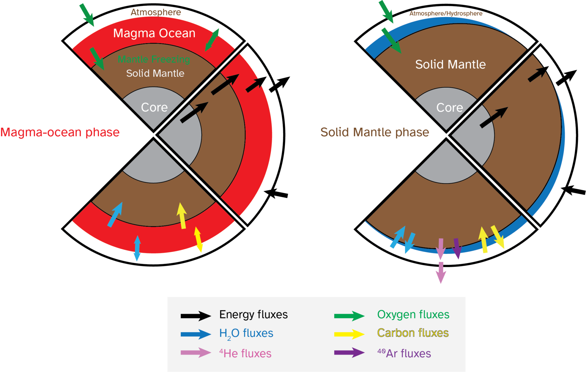
Figure 1: A simplified schematic of the PACMAN model the authors used. On the left is the magma-ocean phase that consists of (from innermost to outermost layer) the core, a solid mantle, magma ocean, and atmosphere. On the right is the solid mantle phase which occurs after the magma ocean solidifies, consisting of the core, solid mantle, and the atmosphere/hydrosphere. Different colored arrows show what components leave and enter each layer in the model. [Adapted from Krissansen-Totton et al. 2021]
There are lots of unknown parameters and initial conditions in the model such as CO2 pressure and planetary albedo (reflectiveness), so the authors run their model 10,000 thousand times to sample all 24 of these unknown parameters. Out of all of these runs, only 10% ended successfully in a state that mirrors Venus’s modern atmospheric and surface conditions and chemical abundances. What’s interesting about these successful models is that they suggest Venus’s current state is compatible with two different histories: some of the models tell us Venus was never habitable in its past, while others claim that Venus was transiently habitable, meaning it could have contained an ocean up to ~100 meters deep on its surface for anywhere between 0.04 and 3.5 billion years before succumbing to the runaway greenhouse effect. The latter scenario should have left salt or mineral deposits on the surface after all the water evaporated, leaving these materials potentially accessible to future remote sensing observations!
And the Winner Is…
So which model is correct? Unfortunately, there is no definitive answer since the authors found that both models are favored under different conditions. CO2 tends to make it difficult for hydrogen to escape if the water concentration is too low. Therefore, in the uninhabitable scenarios where no surface water is present, H2O in the atmosphere has a hard time escaping because CO2 continually dominates the atmosphere instead of being locked in the surface. That means that these scenarios can’t reproduce the modern water-less and oxygen-less Venus that we see today. But, if CO2 is allowed to radiatively cool the upper atmosphere, then water can condense on the surface and CO2 is removed from the atmosphere and stored away in the interior of the planet, giving Venus a chance to have a period of enhanced water loss that can then initiate the runaway greenhouse effect before the CO2 is outgassed back into the atmosphere.
On the other hand, most modern models assume that when the magma ocean phase ends, virtually all the carbon and water from the magma (so-called volatiles) live in the atmosphere. But it is possible that some of these volatiles are trapped in the resulting solid mantle instead. If this is allowed, then far fewer models allow for Venus to have been habitable. This is because it would take longer for water to then be released back into the atmosphere, making it hard to explain Venus’s current almost non-existent water abundance.
The bottom line here is that either of these two scenarios is possible and consistent with modern observations. Which scenario wins depends on our assumptions and model parameters. Though this might seem a bit anticlimactic, understanding and constraining Venus’s evolution is important for interpreting the atmospheres and histories of other exoplanets out there that might have gone through similar processes. JWST might be capable of constraining what the atmospheres of other so-called exo-Venuses are, like some of the TRAPPIST-1 system planets. Hopefully, our studies of both Venus and exo-Venuses can symbiotically help shine a light on planetary evolution!
Original astrobite edited by Ishan Mishra.
About the author, Katya Gozman:
Hi! I’m a second-year PhD student at the University of Michigan. I’m originally from the northwest suburbs of Chicago and did my undergrad at the University of Chicago. There, my research primarily focused on gravitational lensing and galaxies while also dabbling in machine learning and neural networks. Nowadays I’m working on galaxy mergers and stellar halos, currently studying the spiral galaxy M94. I love doing astronomy outreach and frequently volunteer with a STEAM education non-profit in Wisconsin called Geneva Lake Astrophysics and STEAM.


