
Pulsar Discovery from an Enormous Telescope
Magnetized neutron stars in distant globular clusters are a challenge to detect — but it’s a job made easier by the world’s largest filled-aperture radio telescope. Recent high-sensitivity observations have uncovered an erratic new star system.
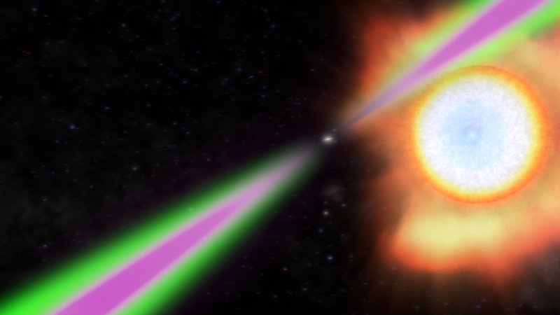
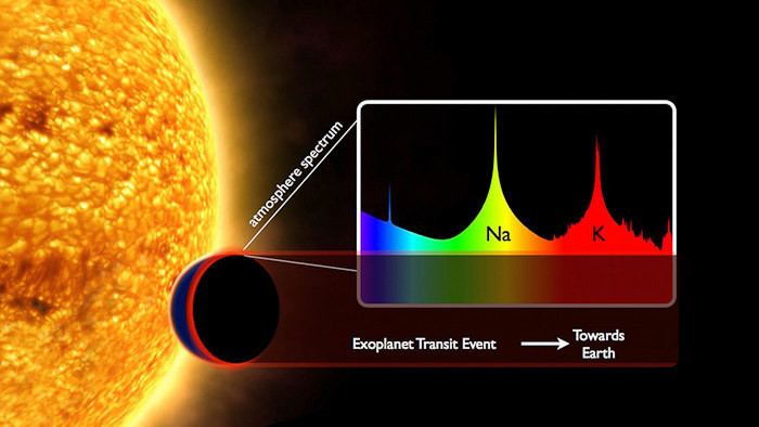
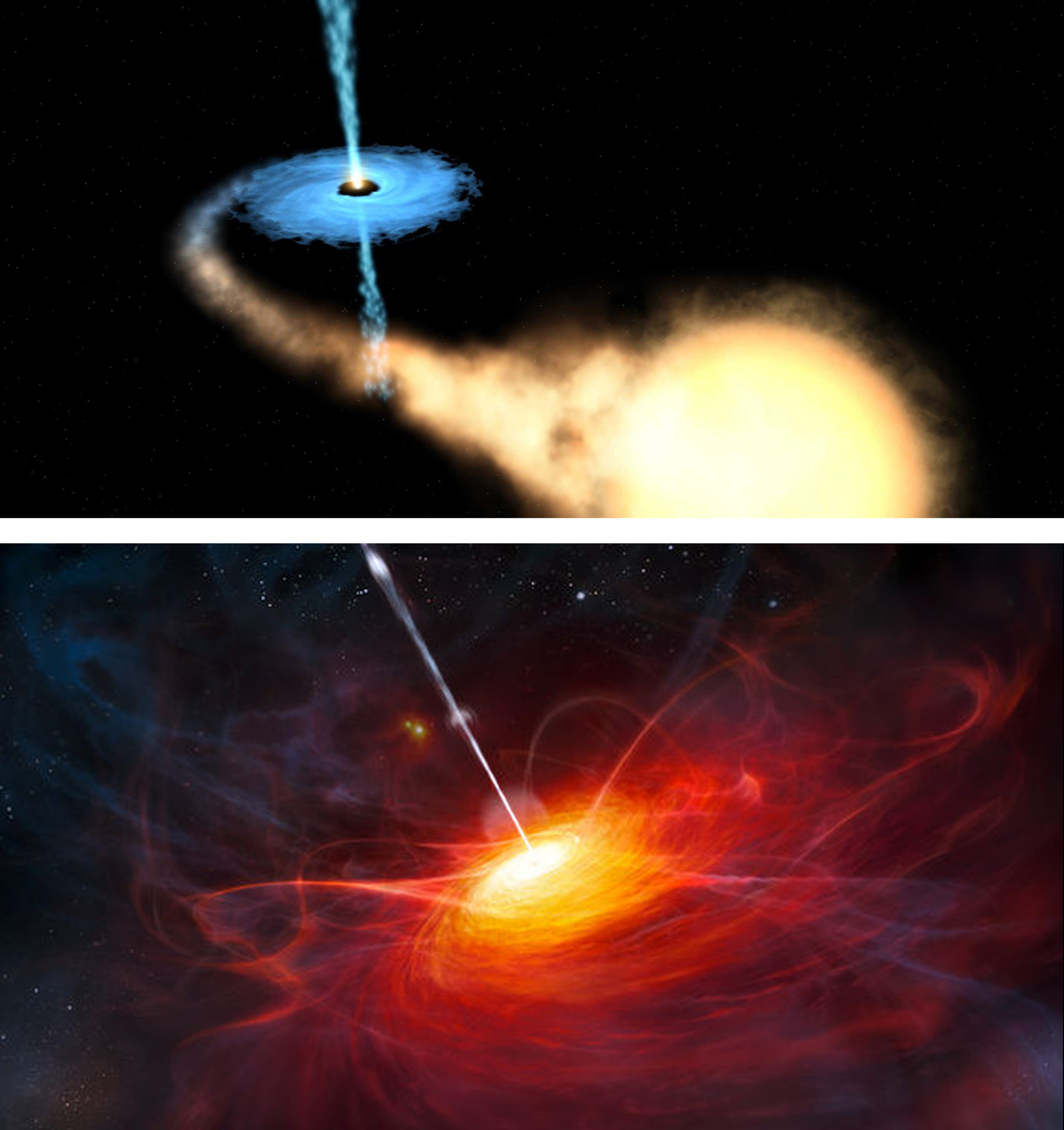
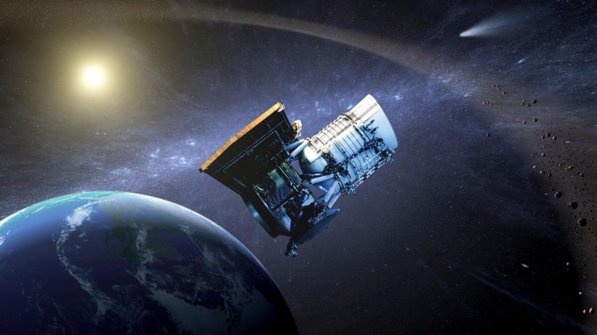
Artist’s illustration of a pulsar (left) and its small stellar companion (right), viewed within their orbital plane. [NASA Goddard SFC/Cruz deWilde]
Pulses from Distant Clusters
Pulsars are the compact remnants of dead stars that shine powerful beams of emission into space as they spin. The brightness of these beams and the regular timing of their pulsations makes pulsars valuable targets for observatories; not only can they tell us about stellar evolution and their environments, but they also serve as probes of the interstellar medium, space-time, and more.
Since the discovery of the first pulsar in 1967, we’ve found thousands of these stellar clocks in our galaxy. While many are located relatively nearby in the galactic disk, we’ve also observed a population of pulsars in the distant globular clusters that orbit the Milky Way. These pulsars are a useful tool for probing a very different environment: the dense stellar cores made up of an old population of stars.
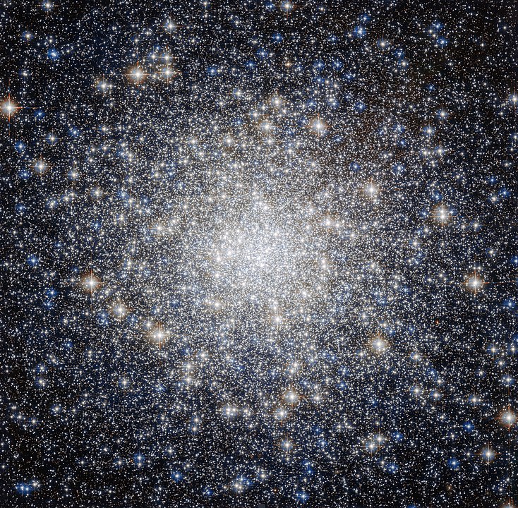
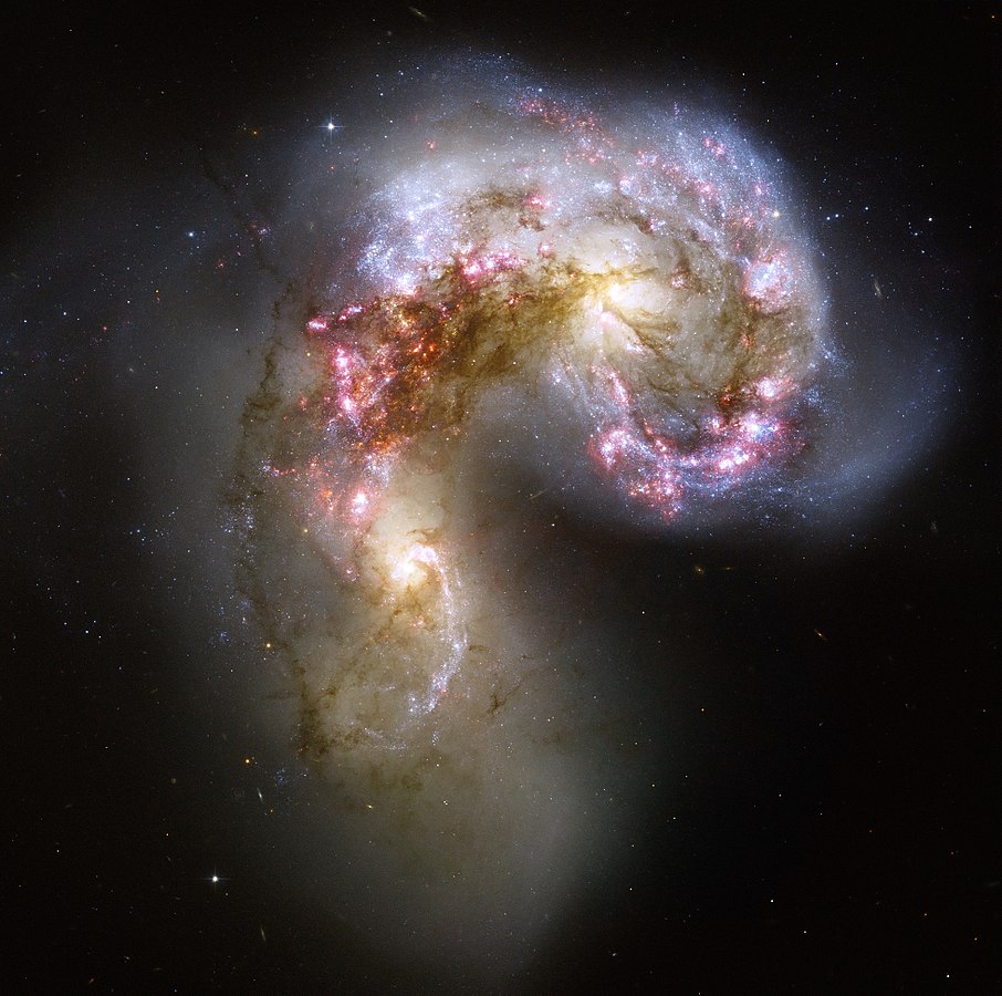
Hubble image of the globular cluster M92. [ESA/Hubble]
A Powerful Telescope
The Five-hundred-meter Aperture Spherical radio Telescope (FAST), built into the hilly landscape in southwest China, is the world’s largest filled-aperture telescope. Its size dwarfs that of the Arecibo Observatory in Puerto Rico, and its dish has the advantage of being shapable — the panels that make up its surface can be tilted by a computer to change the telescope’s focus.

Comparison of the FAST (bottom) and Arecibo Observatory (top) radio dish profiles at the same scale. [Cmglee]
Among them: the first discovery of an eclipsing binary pulsar in globular cluster M92, as reported in a recent publication led by Zhichen Pan (NAO, Chinese Academy of Sciences).
An Exotic System

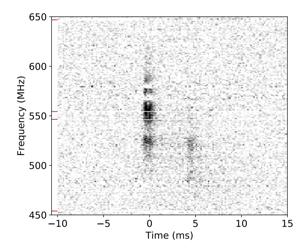
Phase-folded pulse data for PSR J1717+4308A, as observed by FAST (left panel) and by the Green Bank Telescope (right panel). Eclipses are visible as breaks in the data. The difference in sensitivity between the two telescopes is starkly evident. [Adapted from Pan et al. 2020]
This pulsar, PSR J1717+4308A, is in a close (period of 0.20 days) eclipsing orbit with its companion, making it what’s known as a “red-back pulsar”. Radiation from the pulsar has pummeled its companion star, creating a cloud of ionized material that surrounds it and causes the pulsar’s eclipses to vary in duration and timing.
The discovery of this object demonstrates the potential of FAST as a probe of the globular cluster pulsar population. More observations of M92 are planned in the future, as well as observations of dozens of even richer clusters. Keep an eye out for more FAST results as this telescope ramps up operations!
Citation
“The FAST Discovery of an Eclipsing Binary Millisecond Pulsar in the Globular Cluster M92 (NGC 6341),” Zhichen Pan et al 2020 ApJL 892 L6. doi:10.3847/2041-8213/ab799d


.jpg)