Hints of Young Solar Systems
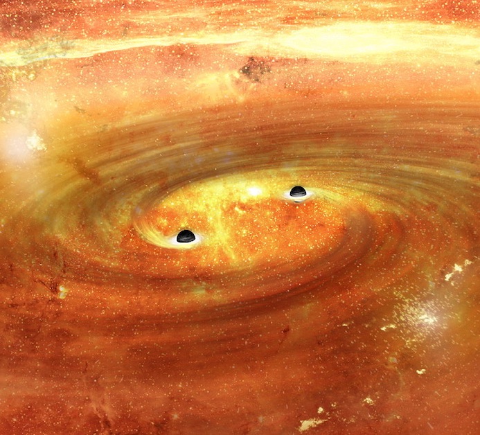
How did our solar system’s planets first form within the swirling disk of gas and dust that surrounded the newborn Sun? One of the best ways to answer this question is watch other solar systems as they form — and the Atacama Large Millimeter/submillimeter Array (ALMA) continues to help us do so.
A History of Large Targets
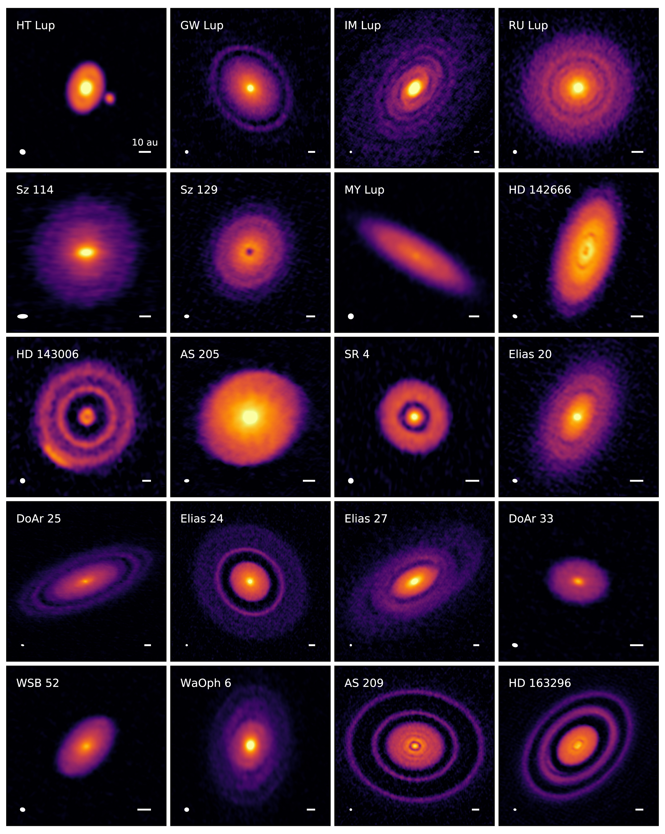
Gallery of 240 GHz (1.25 mm) continuum emission images for the disks in the DSHARP sample. The scale bars in the lower right of each image indicate 10 au. Click to enlarge. [Andrews et al. 2018]
Thus far, however, we’ve mostly focused on imaging the especially large disks that give us the best look at disk substructure. As an example, the Disk Substructures at High Angular Resolution Project (DSHARP) survey used ALMA to image twenty large, bright disks with effective radii — the radius that encompasses 68% of the light from the dusty disk — of ~50 au on average.
But the vast majority of disks are faint, and their dusty disks are much more compact, with effective radii of less than 20 au. Do these more typical disks show the same wealth of substructures that we’ve spotted in larger disks? And what can this tell us about planet formation?
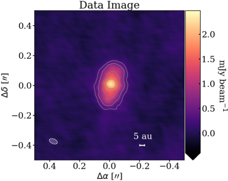
ALMA continuum image of the GQ Lup disk. The scale bar at the lower right indicates 5 au. [Adapted from Long et al. 2020]
Stopping the Migration
In a new study led by Deryl Long (University of Michigan), a team of scientists has used ALMA to explore one of these more typical systems: a compact disk with effective radius of 19 au around the star GQ Lup A. The high angular resolution of ALMA’s observations allow the team to resolve the dust emission even in this small disk, revealing a wealth of substructures very similar to those spotted in larger disks.
What do these substructures tell us? One challenge to planet formation theories is that larger dust grains should migrate inward through the disk in a process called radial drift, accreting onto the star before they can clump together to form planetesimals.
Long and collaborators’ observations of the GQ Lup system suggest that pebble-sized dust grains can be trapped by variations in pressure in the disk, halting the grains’ drift and giving them a chance to clump. This means that small disks may have the same opportunity as large disks to form young planets.
The Birth of a Solar System

Size-luminosity relationship for millimeter continuum sources with disk properties. DSHARP disks are marked with green circles. The new observations of GQ Lup (red diamond) move us toward a discovery space of smaller disks. [Long et al. 2020]
One of the disk gaps identified by the authors lies at ~10 au, which is roughly the distance of Saturn from our Sun. Studying GQ Lup could therefore reveal how planets like Saturn develop from a dusty disk. What’s more, these observations of GQ Lup indicate that there may be a rich population of young solar-system analogs out there, just awaiting discovery and exploration.
Citation
“Hints of a Population of Solar System Analog Planets from ALMA,” Deryl E. Long et al 2020 ApJL 895 L46. doi:10.3847/2041-8213/ab94a8