
Cosmic Rays as the Source of Life’s Handedness
You might expect living cells to be composed of a random soup of materials — but look closely and you’ll find they’re built from molecules with distinct orientation preferences. How did life’s preferred “handedness” arise?
Living Single-Handedly
Billions of years ago, perhaps on the barely solidified crust of young Earth, life somehow arose from non-living matter. Today, we still haven’t solved the puzzle of how this transition from non-living to living occurred — but nature has left behind some helpful clues, including the intriguing geometry of life’s building blocks.
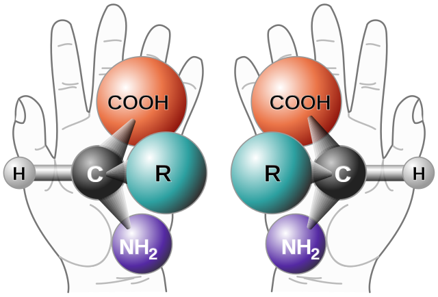
This generic amino acid exists in both a left-handed and a right-handed form: all the same things are attached in the same order, but the two forms are mirror images and cannot be superimposed. If both forms exist, why is life built from only left-handed amino acids? [Public Domain]
But while the pre-biological soup of material on early Earth contained both left-handed and right-handed forms of chiral molecules, living organisms are homochiral: they’re built almost exclusively from left-handed amino acids and right-handed sugars and nucleotides, which preferentially construct right-handed DNA and RNA.
A Cosmic Influence
What determined the handedness of Earth’s life? Was it a random initial disequilibrium — perhaps an overabundance of right-handed nucleotides trapped in a prebiotic nursery — that was then copied to all subsequent life? Or might the bias only have arisen later, driven by an outside source?
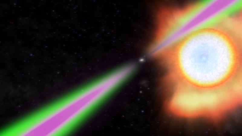
In a new study, scientists Noemie Globus (New York University and Flatiron Institute) and Roger Blandford (Stanford University and KIPAC) explore how cosmic rays may have shaped the evolution of early life forms.
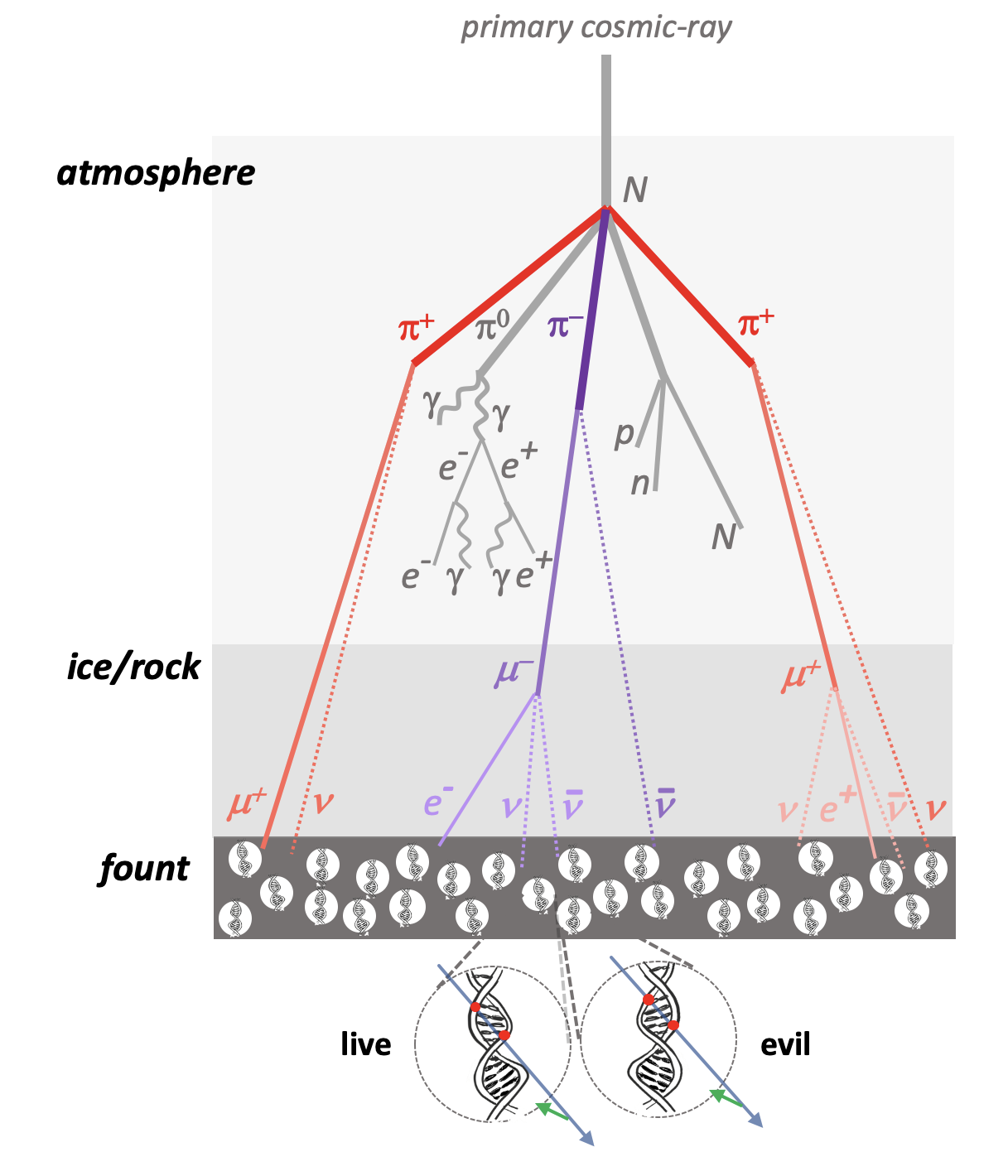
In this schematic, the authors illustrate how the decay of a cosmic ray proton produces a shower of spin-polarized particles. When these particles reach the Earth’s surface, they affect right-handed and left-handed molecules differently, imparting a chirality bias. [Adapted from Globus & Blandford 2020]
Mutating for Survival
Cosmic rays are highly energetic, charged particles that careen in from space and slam into the Earth’s atmosphere, producing a cascade of secondary particles that can reach the planet’s surface.
Irradiation from cosmic-ray cascades is thought to drive gene mutation in DNA — an exploratory process that is critical for evolution. Many successive gene mutations in the earliest stages of life likely allowed proto-life forms to adapt to their environment, increasing their complexity and their chances of survival.
Intriguingly, the physical force that governs cosmic-ray cascades naturally introduces a preferential handedness in the secondary particles that reach the planet’s surface. Could this handedness somehow have introduced homochirality for life forms?
Pick a Hand
Globus and Blandford propose a model in which prebiotic chemistry produced both of the mirror versions of DNA and RNA. As these proto-lifeforms worked to self-replicate and evolve, cosmic rays rained down, introducing minor mutations.
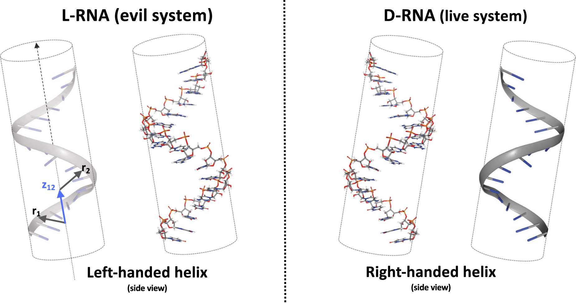
Prebiotic chemistry may have produced both the left-handed and right-handed forms of RNA (which the authors cleverly label “evil” and “live” to underscore their mirror-image nature). [Adapted from Globus & Blandford 2020]
Can we test this model? We might find supporting evidence from laboratory experiments that simulate the influence of cosmic-ray irradiation on bacteria mutation rates. And, of course, we can hope that we’ll one day explore life’s building blocks in samples from asteroids and other planets, further pinpointing what led to life as we know it.
Citation
“The Chiral Puzzle of Life,” Noemie Globus and Roger D. Blandford 2020 ApJL 895 L11. doi:10.3847/2041-8213/ab8dc6


