Features RSS

High-contrast photograph of the stripes and bands of Jupiter’s atmosphere.

As a moon orbits around its planet, the gravitational forces of the two bodies exert mutual pulls on one another. What happens to the inside of a gas-giant planet as a consequence of the tugs of its moons? New data from the Juno orbiter at Jupiter are providing answers!

Types of Tides

We needn’t look far to see how a moon’s gravity can influence its planet: anyone who’s witnessed low or high tide on a beach has experienced the effects of our own Moon.

illustration of the force magnitude and direction at the surface of the Earth as a consequence of the Moon's gravitational pull

The Moon exerts a differential gravitational pull on the Earth that manifests itself as tidal bulges on the sides of Earth facing and opposite the Moon. [Krishnavedala]

This well-known phenomenon is an example of hydrostatic tides: the pull of the Moon’s gravitational field causes the Earth to deform, creating stationary tidal bulges on the sides of the Earth closest to and opposite from the Moon. Since the most easily deformed part of the Earth is its surface water, we see these tidal bulges predominantly in our oceans, with two high tides and two low tides evident each day.

But hydrostatic tides are not the only type of tidal effect that the gravitational pull of moons can create. An additional effect is called dynamical tides, in which the gravitational influence of the moon induces oscillations in the interior of a gaseous planet. These waves could, if detected and understood, be used to probe the inside of the planet to learn about its structure and composition.

Until now, we’ve only detected the effect of hydrostatic tides in gas-giant planets — never the waves from dynamical tides. But new observations from the Juno orbiter are now shaking things up.

illustration of a three-armed spacecraft in front of Jupiter

Artist’s rendering of the Juno spacecraft. [NASA/JPL-Caltech]

A New Probe on the Scene

The Juno probe was launched in 2011, and it arrived at Jupiter and began orbiting this nearby gas giant in 2016. One of Juno’s instruments is designed to map out Jupiter’s gravitational field by making careful measurements of minute changes in Juno’s velocity as it orbits. This detailed mapping allows researchers to detect the tidal response of Jupiter to the gravitational pull of its system of moons.

Intriguingly, Juno’s measurements show a tidal response that can’t be explained exclusively by hydrostatic tides. In a new publication, California Institute of Technology scientists Benjamin Idini and David Stevenson explore whether Juno may, in fact, be seeing evidence of dynamical tides in Jupiter.

Io-Induced Waves

Photograph of Io in front of the face of Jupiter

This photograph, captured by Voyager 1 at Jupiter in 1979, shows Io and its shadow passing across Jupiter’s face. [NASA / JPL / Ian Regan]

Idini and Stevenson use perturbation theory and tidal models to calculate the predicted effect of the dynamical tides excited by Jupiter’s moons. The authors demonstrate that the deviation from hydrostatic equilibrium measured by Juno is consistent with expected dynamical tides induced by Io, the closest-in Galilean moon with the strongest gravitational influence.

The authors’ results suggest that Juno has indeed obtained the first unambiguous detection of the gravitational effect of dynamical tides in a gas-giant planet. Idini and Stevenson hope that we’ll be able to use these results — and future, even higher-precision data from Juno as it continues its extended mission — to explore Jupiter’s interior and answer long-standing questions about the inside of this gas giant.

Citation

“Dynamical Tides in Jupiter as Revealed by Juno,” Benjamin Idini and David J. Stevenson 2021 Planet. Sci. J. 2 69. doi:10.3847/PSJ/abe715

Telescopes are getting better and better at detecting the components of exoplanet atmospheres. But what can those components tell us about a planet’s climate? It turns out that water vapor may be especially useful in this regard.

Atmospheres on Tidally-Locked Planets

The Moon orbiting the Earth, with a yellow arrow showing the direction of the Moon’s rotation. The Moon’s rotational period matches its orbital period so that the same face of the Moon faces Earth at all times. Click to play. [NASA’s Scientific Visualization Studio]

As we find more and more exoplanets, we’re realizing that our solar system may be the exception to the rule! The menagerie of exoplanets we’ve discovered so far includes Jupiter-sized planets that are close to their suns, planets with two suns, and planets that take one orbit about their sun to complete one rotation on their axis — these planets are said to be tidally locked.

Just like our tidally locked Moon always shows the same face to the Earth, tidally locked planets always show the same face to their sun. So, a tidally locked planet will have a consistent dayside and nightside. This has fascinating implications for their climate, and even moreso when we consider that there could be tidally locked Earth-like planets!

A cross section of the planet’s atmosphere with a specific model pressure showing humidity with the colored contours and mass flow with the white contours. The nightside is on the left while the dayside is on the right. [Adapted from Ding & Pierrehumbert 2020]

Models of the water vapor runaway greenhouse effect — when radiation is prevented from efficiently leaving a planet — on tidally locked planets show that the nightside emits more thermal radiation than the dayside as the planet approaches the runaway greenhouse state. Since this reversal of thermal emission requires the emergence of clouds and the buildup of water vapor on the nightside of the planet, spotting it in an exoplanet’s atmosphere could be a useful indicator that the atmosphere is not dry.

To achieve nightside buildup of water vapor, the vapor must avoid being caught on the dayside in a “cold trap”, where it would be cooled, condense, and remain on the dayside. On a planet with inefficient cold trapping, the water vapor can be swept to the nightside to contribute to the thermal emission there.

This weak cold trap effect has mostly been modeled for planets with warm, thick atmospheres, but it is feasible for this effect to also occur on planets with thin, temperate atmospheres. A recent study done by Feng Ding (Harvard University) and Raymond Pierrehumbert (University of Oxford, UK) explores the second scenario for slowly rotating tidally locked planets.

Simulating Two Sides of a Planet

The brightness of the modeled planet as seen at a wavelength of 1,000 cm as it rotates. The different lines indicate different pressures and atmospheric conditions. The black vertical dashed line marks the superior conjunction, where the star is between the observer and the planet. Click to enlarge. [Adapted from Ding & Pierrehumbert 2020]

Ding and Pierrehumbert specifically looked at atmospheres rich in water vapor, which would allow for the necessary clouds and weak cold trap to exist. Their model planet had a period of 40 days and accounted for a variety of interactions that could occur on an Earth-like planet with an atmosphere and oceans. They were also able to vary atmospheric pressure and surface temperature and so modeled several different conditions for their planet.

It turns out that thin, temperate atmospheres with weak cold traps do show the same nightside–dayside emission difference as warm, thick atmospheres as they approach the runaway greenhouse state! Interestingly, the difference between the nightside and dayside emissions can point to the relative amount of water vapor in a planet’s atmosphere as well as the atmospheric pressure — insight we can’t gain from the planet’s transmission spectrum. Further properties of a planet’s atmosphere can be determined by observing how the brightness of the planet changes as it rotates.

The subtleties from this study can’t be picked up by our telescopes yet, but possible future missions like the Origins Space Telescope may be able to. There’s no need to rush though: there are still lots more planets to simulate!

Citation

“The Phase-curve Signature of Condensible Water-rich Atmospheres on Slowly Rotating Tidally Locked Exoplanets,” Feng Ding and Raymond T. Pierrehumbert 2020 ApJL 901 L33. doi:10.3847/2041-8213/abb941

Illustration of two black holes, each surrounded by an accretion disk, merging.

Could the biggest — literally — gravitational-wave discovery yet be something other than what it initially seemed? A new study suggests that the most massive merger of black holes detected by LIGO/Virgo may have included a surprising lightweight.

Echoes of a Surprising Merger

In May 2019, a collision of two black holes shook spacetime, registering in the LIGO and Virgo gravitational-wave detectors as the heaviest black-hole merger discovered yet. Initial analysis of GW190521 suggested that the participants in this cosmic collision were ~85 and ~66 times the mass of the Sun, and that they formed a final black hole of ~142 solar masses — an unexpectedly heavy outcome that lands in the elusive category of intermediate-mass black holes.

Stellar graveyard Nov 2020

The rapidly expanding “stellar graveyard”, a plot of the masses of the different components of observed compact binary mergers. GW190521, top center, is more massive than any other binary merger we’ve observed. [LIGO-Virgo/Northwestern U./Frank Elavsky & Aaron Geller]

But GW190521 raised eyebrows for another reason as well: the estimated masses of the two merging black holes fell between 65 and 120 solar masses, a region known as the pair-instability mass gap. This range of masses should be inherently off-limits for black holes born from collapsed stars, based on our current understanding of stellar evolution processes.

While there are many hypotheses about how mass-gap black holes could potentially form, two scientists have focused on an alternative angle: what if we were simply wrong in our estimate of GW190521’s component masses?

Checking Our Assumptions

How do we measure component masses from a gravitational-wave signal? Decades of theoretical research have produced a vast array of model signals for mergers with different parameters. By comparing the observed gravitational-wave signal to the various models, we can calculate which ones fit best. But this comparison relies on what are called priors — a set of assumptions that go into the analysis and affect the outcome.

Three plots showing the GW190521 signal at Hanford, Livingston, and Virgo

The observed gravitational-wave signal of GW190521 in each of the three detectors (black), plotted with two best-fit models: one for when the component mass ratio is between 1 and 2 (blue) and one for a mass ratio between 2 and 25 (orange). [Nitz & Capano 2021]

In a recent publication, scientists Alexander Nitz and Collin Capano (Max Planck Institute for Gravitational Physics and Leibniz University Hannover, Germany) reanalyze the gravitational-wave signal for GW190521 using a different set of priors and constraints than the original analysis completed by the LIGO collaboration.

Nitz and Capano find that their analysis admits two possible solutions for GW190521: one similar to that found by the LIGO collaboration — and another, in which the component black holes are ~16 and ~170 solar masses. This second option becomes even more heavily favored when the authors analyze the gravitational-wave signal simultaneously with an electromagnetic flare that may have been associated with the merger.

An Uneven Pair?

What does this outcome tell us? The masses in Nitz and Capano’s second solution both lie outside of the pair-instability mass gap, neatly resolving the paradox previously created by this merger.

If the authors’ interpretation is correct, then GW190521 would represent the first detected intermediate-mass-ratio inspiral — a type of merger in which one component is substantially larger than the other. This signal then provides an exciting milestone and an opportunity to learn more about the different types of dramatic collisions that occur in our galaxy.

Citation

“GW190521 May Be an Intermediate-mass Ratio Inspiral,” Alexander H. Nitz and Collin D. Capano 2021 ApJL 907 L9. doi:10.3847/2041-8213/abccc5

illustration of flow lines with kinks in them streaming off of the sun

Parker Solar Probe

Artist’s illustration of the Parker Solar Probe. A special ApJS issue features around 50 articles detailing early results from this mission. [NASA/Johns Hopkins APL/Steve Gribben]

On its first journey dipping into the Sun’s outermost atmosphere — the extended corona — the Parker Solar Probe detected something unexpected: strange kinks in the streams of plasma flowing off of the Sun. Scientists have since developed a detailed explanation for the unusual behavior the probe found.

A Kink in the Plan

Launched in 2018, the Parker Solar Probe (PSP) is on a mission to orbit the Sun, dipping ever deeper into our star’s outer corona to make measurements of the magnetic field and plasma conditions there. The probe is currently approaching its eighth perihelion pass, where it will graze an altitude just 15 solar radii or so above the Sun’s surface! But the PSP was already making surprising detections on its very first perihelion pass in 2018.

switchbacks

Animation of magnetic switchbacks propagating outward through the corona. [NASA’s Goddard Space Flight Center/Conceptual Image Lab/Adriana Manrique Gutierrez]

The solar wind — a flow of charged particles that streams off of the Sun — travels radially outward into the solar system on large scales. But close to the Sun, the PSP found, the wind’s flow structure is more complex. PSP flew through what are termed switchbacks: S-shaped hitches in the flow lines that propagate outward, representing sudden changes in magnetic field orientation and plasma velocity.

The discovery of this phenomenon put theorists to work. What causes switchbacks, and what might they tell us about the production of the solar wind and plasma processes around the Sun? In a study led by Gary Zank (University of Alabama in Huntsville), a team of scientists present a model that may explain these strange phenomena.

Searching for (Re)connection

three-panel diagram illustrating the stages of interchange reconnection and switchback production

Diagram of the authors’ model for production of switchbacks by interchange reconnection: a) a closed coronal loop and open magnetic field lines approach each other; b) the first field line reconnects, producing an open field line with an S-shaped structure; c) the switchback is launched, propagating both upward and downward, as a new reconnection event begins on the next field line. [Adapted from Zank et al. 2020]

In Zank and collaborators’ model, switchbacks originate high in the solar corona. There, coronal loops — loops of magnetic field anchored in the Sun’s photosphere and arcing up into the corona — extend out to large distances (~6 times the radius of the Sun!). When these loops move near open magnetic field lines in the solar wind, a process called interchange reconnection can occur, in which the magnetic field lines of the coronal loop suddenly break and then reattach themselves to the lines of the open field, forming a lower-energy configuration and releasing a burst of plasma.

The authors derive the mathematical theory describing how a switchback produced from this reconnection would propagate through the inhomogeneous solar corona. The reconnection event launches magnetic field deflections both out into the solar system and down toward the solar surface. The authors show that the most extreme of these deflections take the form of the S-shaped structures that PSP observed as the most dramatic switchbacks.

Matching Theory to Observation

Zank and collaborators demonstrate that their model is both qualitatively and quantitatively consistent with PSP’s observations of switchbacks in its first perihelion pass. Not only does the theory well reproduce a single switchback, but it also shows how interchange reconnection events can occur in quick succession for loops made of multiple magnetic field lines, resulting in clustering of switchbacks consistent with PSP’s measurements.

We’re still in early stages of understanding these strange phenomena, but more help is on the way! PSP continues to amass a vast trove of data as it repeatedly swings through the Sun’s atmosphere — which we can hope will soon bring the mystery of switchbacks to a close.

Citation

“The Origin of Switchbacks in the Solar Corona: Linear Theory,” G. P. Zank et al 2020 ApJ 903 1. doi:10.3847/1538-4357/abb828

Illustration of a bright flash of light surrounded by ripples that represent gravitational waves

Collisions of neutron stars and black holes provide insights beyond stellar evolution: these mergers may also be the key to unlock precise measurements of the cosmological parameters that describe our universe. A recent study explores what we can hope to learn with multimessenger cosmology in the next few decades.

Pinning Down Parameters

Measurements of the Hubble constant via different methods over time. The Cepheid method suggests that the Hubble constant is around 73 km/s per megaparsec while the CMB value is around 67 km/s per megaparsec. The TRGB method falls between the other two. Prior to about 2013, the Cepheid and CMB values fell in each other’s realm of error.

Measurements of the Hubble constant via different methods show a discrepancy in measured value that has only grown over time. [Freedman et al. 2019]

Obtaining precise measurements for cosmological parameters is critical as we attempt to understand the origins, the evolution, and even the composition of our universe. Estimates of figures like the Hubble parameter (H0), the matter density parameter (Ωm), and the dark energy equation of state parameter (w) abound.

Unfortunately, different measurement techniques produce a wide spread in values for these parameters. Scientists have long waited for a new, independent approach that will provide a resolution to the tension between past measurements. Now, in the age of gravitational astronomy, we have one: the standard siren technique.

diagram illustrating 4 stages of a neutron-star merger.

Diagram illustrating the stages of a neutron-star collision. In the model, 1) two neutron stars inspiral, 2) they merge and produce a gamma-ray burst lasting a tenth of a second, 3) a small fraction of their mass is flung out and radiates on timescales of weeks as a kilonova, 4) a massive neutron star or black hole with a disk remains after the event. [NASA, ESA, and A. Feild (STScI)]

Insights from Sirens

We’ve previously discussed the use of dark sirens — black hole–black hole mergers — as a tool to measure cosmological parameters. Standard sirens — the mergers of neutron stars with either black holes or other neutron stars — are a similarly useful tool, but they rely on multimessenger observations rather than only gravitational waves.

The idea is straightforward: by simultaneously observing the gravitational-wave and electromagnetic signals from these explosive mergers, we can obtain both an absolute distance scale and a redshift measurement for the source. This combination allows us to obtain an independent measurement of cosmological parameters — and the more of these joint detections we make, the more precise our measurements will be.

But implementing this approach efficiently requires some planning. What’s the best observing strategy to ensure we can pin these parameters down with the gravitational-wave and electromagnetic observatories planned for the next few decades? A new study led by Hsin-Yu Chen (Harvard University and MIT) explores this question.

The Promise of Future Detectors

schematic timeline of current and future observatories

Schematic timeline of existing (solid), funded (hatched), and proposed (open) GW and EM facilities over the next three decades. Swift+/Swift++ are hypothetical future gamma-ray satellites. [Chen et al. 2021]

Chen and collaborators evaluate the impact of a number of expected future observatories. These include:

  1. Three eras of gravitational-wave detectors with increasing sensitivity (A+, Voyager, and Cosmic Explorer)
  2. Wide-field survey telescopes like the Vera Rubin Observatory that can detect kilonovae, the optical and infrared counterparts of mergers involving neutron stars.
  3. High-energy observatories like Swift and its successors to detect short gamma-ray bursts, a highly directional but bright counterpart to mergers.
Plot showing the uncertainty on H0 using different observing campaigns that combine future observatories.

Uncertainty in the measurement of H0 for a variety of different observing strategies. Orange bars indicate the fraction of total observing time available to VRO for each kilonova scenario. [Adapted from Chen et al. 2021]

Based on the capabilities and limitations of these observatories, Chen and collaborators estimate how many mergers we’ll be able to detect via joint gravitational-wave and electromagnetic observations each year with different observing campaigns and demonstrate what constraints these detections will place on cosmological parameters.

Using these calculations, the authors outline an observing strategy for the next three decades. They demonstrate that with clever use of resources, we could soon reach sub-percent-level precision on H0 and tight constraints on the amount and form of dark energy in the universe. This work shows the great potential ahead using standard sirens for precision cosmology.

Citation

“A Program for Multimessenger Standard Siren Cosmology in the Era of LIGO A+, Rubin Observatory, and Beyond,” Hsin-Yu Chen et al 2021 ApJL 908 L4 6. doi:10.3847/2041-8213/abdab0

Illustration of stellar orbits around a central point, with a large gas cloud being torn apart in the foreground.

In 2019, the supermassive black hole at the center of our galaxy woke up and emitted a series of burps. A new study now examines what meal may have led to this indigestion.

Active Galactic Nucleus

Artist’s impression of the dramatic outflows from an active galaxy’s nucleus. The Milky Way’s supermassive black hole, in contrast, is very quiet. [NASA/SOFIA/Lynette Cook]

Waking Up for a Snack

Sgr A*, the 4.6-million-solar-mass black hole that lies at the center of the Milky Way, is normally a fairly quiet beast. The black hole slowly feeds on accreting material in the galactic center — but this food source is sparse, and Sgr A*’s accretion doesn’t produce anything like the fireworks we associate with supermassive black holes in active galaxies.

In May 2019, however, Sgr A* suddenly became substantially more active than usual, producing an unprecedented bright, near-infrared flare that lasted roughly 2.5 hours. This flare was more than 100 times brighter than the typical emission from Sgr A*’s casual accretion, and more than twice as bright as the brightest flare we’ve ever measured from our neighborhood monster.

The May 2019 flare marked the start of prolonged increased activity — an unusual number of strong flares that continued at least throughout 2019 (currently analyzed data extends only to the end of that year). What caused Sgr A* to wake up? And do we expect more flaring ahead? A new study by Lena Murchikova (Institute for Advanced Study) explores the options.

Shedding Sources

Photograph of the galactic center with reconstructed orbits of several stars plotted on top.

Reconstruction of the orbits of several S stars at the center of the galaxy. The two colored orbits mark two stars with the closest known approaches to Sgr A*. [Keck/UCLA Galactic Center Group]

Sgr A*’s flares likely came from an abrupt increase in the amount of material available to accrete onto this black hole. Murchikova identifies two likely sources of this excess material.

  1. Shedding S stars
    The dense nucleus of our galaxy hosts a population of stars on tight orbits around Sgr A*. These stars shed mass via stellar winds, and when the stars swing close around Sgr A* at the pericenter of their orbit, this shed mass could accrete onto Sgr A*.
  2. Disintegrating G objects
    Also known to orbit close to Sgr A* are so-called G objects. These extended sources may be gas clouds, stars, or a combination of the two — we’re not sure yet! Tenuous G objects lose mass as a result of friction as they orbit, exhibiting higher rates of mass loss as they get closer to Sgr A* and are stretched out into shapes with large surfaces areas passing through dense background material. The mass they lose through this disintegration at pericenter could then accrete onto Sgr A*.
Photograph of the galactic center showing the positions and estimated orbits of several objects.

The objects G2 (colored red) and G1 (colored blue) and the star S2 are visible in these high-resolution images of the galactic center, taken in 2006 (left) and in 2008 (right). The position of Sgr A* is marked with an X. [MPE/Very Large Telescope]

Short-Lived or Long-Term?

Through a series of calculations, Murchikova estimates how much material is shed by these two types of objects and how long it would take that material to accrete onto Sgr A*. Based on the available observations, the author finds that the most likely explanation for our black hole’s unexpected rumblings in 2019 is currently accreting material from the combined past pericenter passages of the objects G1 and G2.

If this interpretation is correct, we would expect to see flaring continue for a limited time, but Sgr A* should then return to its quiescent state. If the flaring was instead a part of normal variability in the flow of accreting material onto Sgr A*, we would expect the activity to continue for years to come. Continued observations of this rumbling giant will tell!

Citation

“S0-2 Star, G1- and G2-objects, and Flaring Activity of the Milky Way’s Galactic Center Black Hole in 2019,” Lena Murchikova 2021 ApJL 910 L1. doi:10.3847/2041-8213/abeb70

Galactic cosmic rays consist of highly energetic particles coming from sources outside our solar system. The particles that make up these rays have some electric charge, so when the rays enter our solar system they are affected by the Sun’s magnetic field. But how much influence does the Sun actually exert on galactic cosmic rays?

The Sun’s sphere of influence as it travels through the interstellar medium, with the heliosphere, heliopause, and heliosheath marked. The Voyager spacecraft are also shown. The blue circle around the Sun shows the termination shock, where the solar wind goes from supersonic to subsonic speeds. [NASA/JPL-Caltech]

Making Space with Magnetic Fields

The Sun is a mighty presence, and that’s not just in terms of its gravitational influence! With the solar wind, the Sun carves out a roughly elliptical region in the interstellar medium that extends at least 11 billion miles in one direction (for context, the Earth is usually 93 million miles from the Sun). This region is called the heliosphere.

The Sun is able to create the heliosphere thanks to its powerful magnetic field. A quirk of this magnetic field is that its poles switch every 11 years or so, corresponding to what we call the solar cycle. This is a very short timescale when it comes to astronomical phenomena, so with the right instruments, we could study how the Sun’s changing magnetic field affects the passage of charged particles like those in galactic cosmic rays, and how that effect changes with time. 

We can detect galactic cosmic rays using Earth-based observatories, but we’re limited in that we can only see these rays as they appear at 1 astronomical unit (au) from the Sun. But what if we had another galactic ray observatory in a different part of the solar system?

The Cassini spacecraft happens to fit the bill! In a recent study, researchers led by Elias Roussos (Max Planck Institute for Solar System Research, Germany) used Cassini data to augment Earth-based observations of galactic cosmic rays and determine how these rays travel through the solar system over time.

The particle flux as measured by Cassini and the Earth-based observatories over time. The normalization point indicates when all the observatories were at roughly 1 au from the Sun. [Adapted from Roussos et al. 2020]

Cosmic Rays as Seen by Cassini and Others

The Cassini spacecraft observed Saturn from 2004 to 2017, putting it at 9.5 au from the Sun during its mission. One of Cassini’s instruments was the Low Energy Magnetospheric Measurement System (LEMMS), which could measure galactic cosmic ray fluxes. LEMMS has been used in cosmic ray studies before, but Roussos and collaborators made sure to utilize LEMMS data that was taken during Cassini’s flyby of Earth on its way to Saturn. This allowed them to compare the LEMMS data taken at 1 au to data taken at Earth-based observatories.

Aside from Cassini, Roussos and collaborators also used data from the Payload for Antimatter Matter Exploration and Light-nuclei Astrophysics (PAMELA), the Alpha Magnetic Spectrometer-2 (AMS-02), the Balloon-Borne Experiment with a Superconducting Spectrometer (BESS), and BESS-Polar. Luckily, BESS happened to be operating around the time of Cassini’s flyby, allowing for even better calibration of the LEMMS data.

The galactic cosmic ray gradient over time. The shaded rectangles highlight regions where gradient “enhancement” is seen. [Adapted from Roussos et al. 2020]

An Evolving Gradient

The specific quantity Roussos and collaborators wanted to track over time, as the Sun’s magnetic field changed, was the radial intensity gradient of galactic cosmic rays: how the strength of rays varies with distance from the Sun. The data they used were taken over one solar cycle, with 2006–2014 corresponding to negative polarity in the Sun’s magnetic field and 2014–2017 corresponding to positive polarity. 

Roussos and collaborators found that during negative polarity, the galactic cosmic ray gradient is roughly 3.5–4% per au, while during positive polarity it drops down to 2% per au. The gradient reached 4% per au during what we call solar maximum, when the Sun shows the most surface activity during the solar cycle. Yearly to biennial variations in the gradient were also observed.

Roussos and collaborators noted that their measurements of the galactic cosmic ray gradient weren’t meant to be prescriptive of all solar cycles and particles — just the observed solar cycles and protons with specific energies. However, spacecraft like the Mars orbiters and New Horizons will offer even more insight into galactic cosmic rays. So stay tuned!

Citation

“Long- and Short-term Variability of Galactic Cosmic-Ray Radial Intensity Gradients between 1 and 9.5 au: Observations by Cassini, BESS, BESS-Polar, PAMELA, and AMS-02,” Elias Roussos et al 2020 ApJ 904 165. doi:10.3847/1538-4357/abc346

Photo of an edge-on galaxy encircled by a faint stream of stars.

The Milky Way is enwreathed in long streams of stars that hold clues to everything from our galaxy’s history to the nature of dark matter. New research has now identified the likely origins of some of these subtle ribbons.

Streams Across the Sky

Plot showing 23 stellar streams in orbital phase space.

The orbital energy vs. angular momentum of the stars in 23 of the Milky Way’s stellar streams (colored and labeled data), as compared to field stars (black data). [Bonaca et al. 2021]

Stellar streams are associations of stars that are grouped into elongated filaments arcing around a host galaxy. These filaments are thought to be produced when a stream progenitor — like a globular cluster or a satellite dwarf galaxy — is disrupted by its host galaxy’s tidal forces. Stars are drawn out from the progenitor into a tidal stream that then orbits the host galaxy; the progenitor itself may remain connected to the stream, orbit separately, or disrupt entirely.

We’ve observed stellar streams in other galaxies (like NGC 5907, shown above), but we needn’t look that far away — our own Milky Way is host to more than 60 catalogued streams. Of these thin trails, only a handful have been connected to a known progenitor, like a surviving globular cluster. The rest have unknown origins, leaving a number of open questions that only now, with current observations, have answers within reach.

In a recent study led by Ana Bonaca (Center for Astrophysics | Harvard & Smithsonian), a team of scientists has leveraged the incredible precision of the Gaia space observatory to hunt for the origins of 23 cold stellar streams in the Milky Way halo.

Orbital phase space plot showing locations of streams and possible progenitor galaxies and clusters.

Locations in orbital phase space of the 23 stellar streams, labeled by whether they have a dwarf galaxy progenitor (pentagon) or globular cluster progenitor (star). Only one stream, Svöl, falls into the region associated with possible in situ formation (rather than having been brought in via a dwarf galaxy). [Adapted from Bonaca et al. 2021]

A Disrupted Home

Bonaca and collaborators make use of improved proper motions provided in Gaia’s Early Data Release 3 for stars in these 23 streams. By analyzing the energies and 3D angular momenta of these streams, and by examining how the streams are distributed in physical space, the authors are able to identify the probable progenitors for most of the streams.

According to the authors’ results, only 1 of the streams plausibly originated from a globular cluster that was born in the Milky Way. The vast majority instead originated from dwarf galaxies that the Milky Way has accreted. Some of the streams were produced from the dwarf galaxies themselves; others were likely formed from disrupted globular clusters that orbited those dwarf galaxies.

Several of the 23 streams have similar properties, suggesting that many originated from the same progenitors. The authors identify original host dwarf galaxy candidates for 20 of the streams, and they point to 6 specific globular clusters as the origin of 8 of the streams.

Illuminating Dark Matter

Sky map showing locations of 8 stellar streams.

Sky map showing the 6 globular clusters (crosses) that the authors associate with 8 stellar streams (circles). [Adapted from Bonaca et al. 2021]

What can we do with this information? Understanding the origin of these stellar streams allows us to better trace their paths, how long they’ve been orbiting, and what other gravitational interactions they may have had over time. These details are valuable not just for understanding galaxy evolution, but also for mapping out the big-picture distribution of dark matter in our galaxy and studying the small-scale structure of dark matter in the streams’ host galaxies.

Further expansion of Bonaca and collaborators’ work to the other stellar streams orbiting the Milky Way will rely on continued high-quality proper motion measurements of these faint and distant sources. Look for more results as future Gaia data is released!

Citation

“Orbital Clustering Identifies the Origins of Galactic Stellar Streams,” Ana Bonaca et al 2021 ApJL 909 L26. doi:10.3847/2041-8213/abeaa9

Photo of the craters on mars's surface.

On 4 March 2021, the Perseverance rover began rolling through Jezero crater on the surface of Mars. How old is the terrain it’s exploring? A recent study provides an updated answer.

An Impactful History

Photo of the surface of mars centered around Jezero crater.

The landing site of the Perseverance rover on the floor of the Jezero crater. [NASA/JPL-Caltech/University of Arizona]

On Earth, we can determine the ages of surfaces by physically interacting with them. To establish how old a region is, we take a sample of the surface rocks and measure the decay of naturally occurring radiative isotopes within the sample; this technique allows us to identify the rocks’ absolute age. 

But how do we analyze the ages of more distant surfaces that we can’t touch, like planetary bodies in our solar system? This is where impact craters come in. Throughout their lifetimes, bodies in our solar system are peppered with small and large impactors that leave their mark in the form of impact craters. We can use these signatures to build a crater chronology — a timeline that allows us to interpret the ages of different surfaces on a body.

Photograph of a basalt rock in a display case

Lunar olivine basalt, collected by the crew of Apollo 15 and brought back to Earth. [Wknight94]

Building a Timeline

Relative aging of cratered surfaces is straightforward: older surfaces have a higher density of craters than newer ones, because older surfaces have had more time to be bombarded by rocky impactors. Areas of newer geology — for instance, where a lava flow resurfaced a region — have had less time to accumulate impact craters.

But how do we anchor these relative ages in an absolute timescale? That gets trickier. To start with, we need a calibration point. The Moon is ideal for this: we’ve brought back samples of lunar rocks and radiometrically dated them. These absolute dates then provide anchor points that allow us to establish a chronology for the lunar surface.

The Crux Is the Flux

To extrapolate this chronology to other bodies in our solar system — like Perseverance’s new home, Mars — we need two main things: good observations of the body’s crater counts, and an understanding of how the flux of impactors of different sizes has evolved over our solar system’s history.

Two maps showing simulated crater distribution on Mars's surface.

These two simulated crater maps represent different potential bombardment histories for Mars: the top represents an early heavy bombardment ~4.5 billion years ago, and the bottom represents a late heavy bombardment ~4.1 billion years ago. [Marchi 2021]

This latter point is especially challenging. Our best guess as to the past fluxes of different populations of impactors depends on our understanding of the dynamical evolution of the early solar system; as our models change, so do the estimated fluxes. In a new study, scientist Simone Marchi (Southwest Research Institute) has used the latest dynamical models to update Mars’s crater chronology.

Traversing Old Terrain

Marchi’s updated timelines change our predicted ages for Mars’s surface — including for the crater that Perseverance is now exploring. According to the author’s chronology, the dark regions of Jezero crater may be ~3.1 billion years old, which is up to 0.5 billion years older than was previously thought.

Mars’s crater chronology will doubtless be updated again as we continue to improve our models. But we have another prospect for anchoring this planet’s timeline: Perseverance’s goals include caching samples for future return to Earth. If successful, we’ll eventually have some Mars rocks on hand for radiometric dating, providing valuable insight into our solar system’s evolution.

Citation

“A New Martian Crater Chronology: Implications for Jezero Crater,” Simone Marchi 2021 AJ 161 187. doi:10.3847/1538-3881/abe417

Four images of the event horizon of a black hole, with lines drawn in to show the encircling magnetic fields.

Almost two years ago, the Event Horizon Telescope team grabbed the world’s attention with a stunning first picture of the inner regions around a supermassive black hole. Now the team is sharing new insight from their unprecedented observations.

A Giant Telescope’s Target

Four photos of a bright ring of emission around a black hole's shadow.

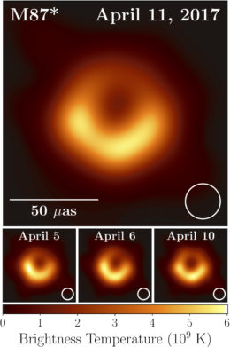
EHT observations of M87 taken over 4 days revealed a bright, asymmetric ring; north is up and east is left. [EHT Collaboration et al 2019]

The Event Horizon Telescope (EHT), a joint network of observatories spanning the globe, recently published its first images of the supermassive black at the center of the nearby active galaxy M87. This series of 4 images, captured in April of 2017, revealed an eerie, glowing ring of hot, magnetized plasma at the event horizon surrounding the “shadow” of the black hole M87*.

Why target M87*? This black hole is relatively nearby, it’s enormous (6.5 billion solar masses!), and it doesn’t vary too quickly. What’s more, M87* is the source of a spectacular, 5,000-light-year-spanning jet.

Looking for Launch

Jets are produced when accreting material is flung out from the poles of a supermassive black hole at incredible speeds — but the means by which they are launched, accelerated, and shaped, and even how they emit light, are all still open questions.

Could M87 help us to better understand these dramatic phenomena? The EHT team has now released two exciting new publications that provide additional insight into the environment close around M87*, from which its jet originates.

Photograph of a long, narrow jet emitted from a bright source.

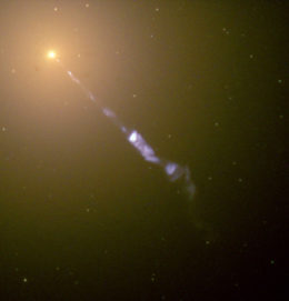
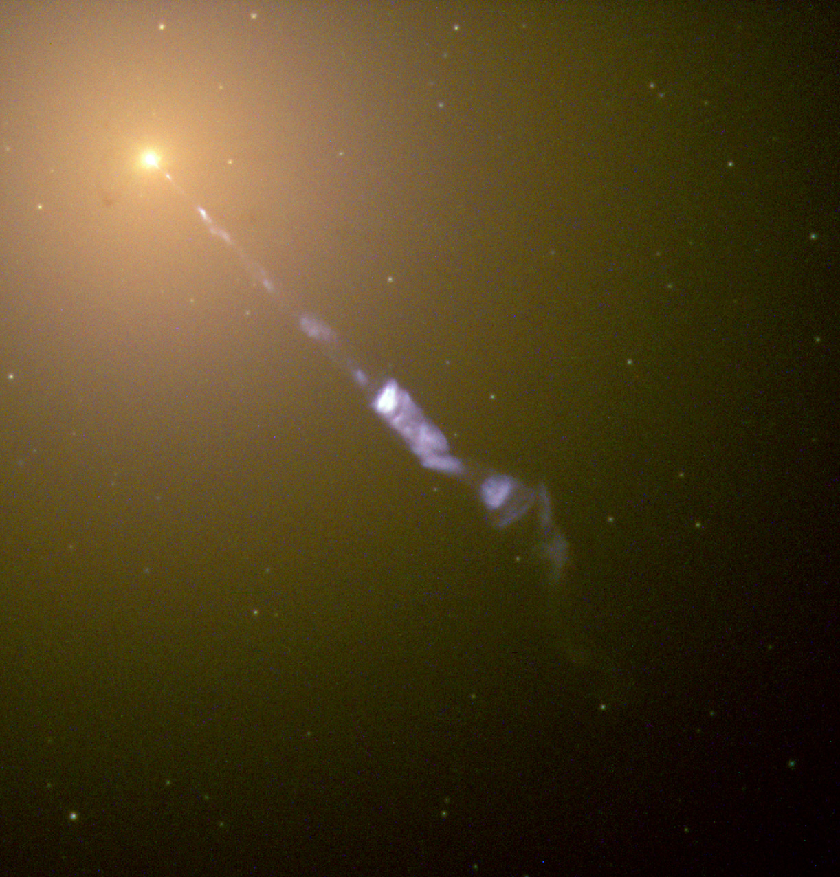
M87’s supermassive black hole produces a collimated jet, visible in this Hubble image. Its counter-jet isn’t seen because relativistic effects make the receding jet appear less bright. [The Hubble Heritage Team (STScI/AURA) and NASA/ESA]

An Added Dimension

When the EHT observed M87* in 2017, it didn’t just capture the data that led to the total intensity images we’ve all seen; it also captured information about the polarization of the light observed.

When light is emitted from hot, magnetized plasma, it is linearly polarized — the magnetic field leaves an imprint on the direction the electromagnetic waves oscillate. As the light travels, this polarization can then rotate or become scrambled as it moves through magnetized matter.

The direction and amount of polarization that we ultimately observe from a source like M87* — if properly disentangled and analyzed — reveals information about the structure of the magnetic fields and the plasma properties close around this black hole.

What We Found and What It Means

Four polarization maps for M87*.

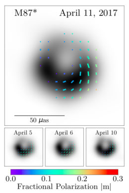
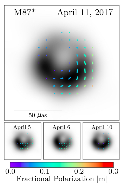
Polarization maps of M87* captured by the EHT on 4 different days. The ticks show the polarization direction and fraction. [EHT Collaboration et al. 2021]

The EHT team’s carefully constructed polarized intensity maps around M87*’s shadow provide a few key insights:

  1. The emission ring around the black hole exhibits polarization, but the polarization fraction is relatively low.
    This confirms the picture of a hot, magnetized plasma in the inner regions around the black hole, and it indicates that the polarization is scrambled inside the emission region, on scales smaller than the telescope can resolve.
  2. Across the 4 different observations spanning roughly a week, the polarization evolves.
    These changes over time are expected, and while the team doesn’t analyze it here, this evolution will likely help us to further constrain models in the future.
  3. In all observations, the polarization pattern is largely azimuthal, wrapping around the black hole.
    This is important: this directionality places significant limits which models can feasibly describe the structure of the magnetic fields and the accretion flow immediately around the black hole.

A MAD Flow?

The authors compare the observed polarization maps for M87* to a gallery of 72,000 snapshot images from numerical simulations probing 120 different models of the accretion flow and jet. The tight constraints from the EHT’s intensity and polarization observations dramatically reduce the set of feasible models, suggesting that the surroundings of M87* are best described by a model called a magnetically arrested disk (MAD).

schematic illustrating magnetic field lines threading through an accretion disk

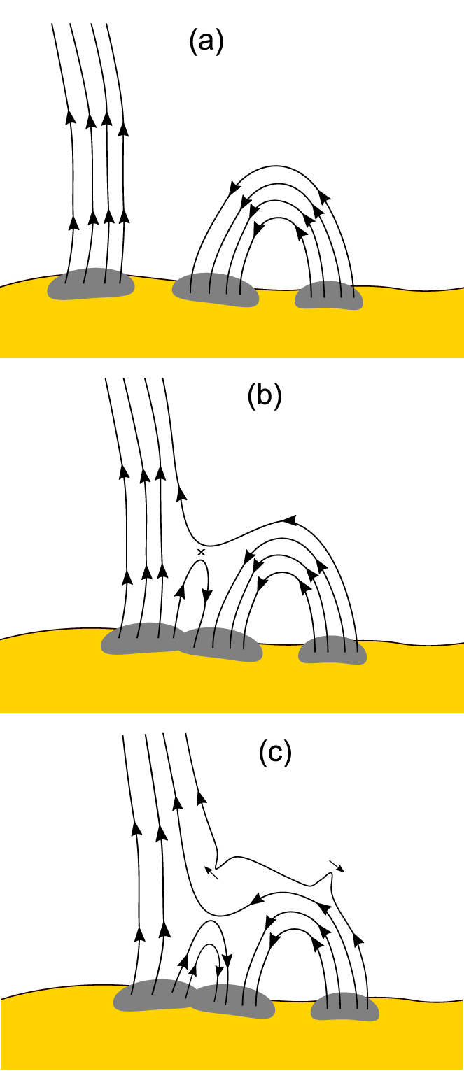
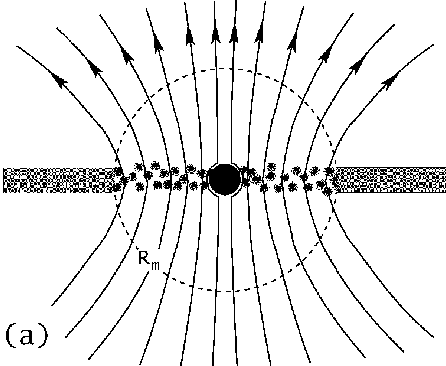
Schematic illustrating the MAD model, as viewed from within the plane of the accretion disk around a black hole. Poloidal magnetic field lines pile up close to the black hole, pushing back on the infalling matter. [Narayan et al. 2003]

In the MAD model, piled-up poloidal magnetic fields close to the black hole are strong enough to affect how matter accretes onto the black hole. This influence and the arrangement of magnetic fields implied by this model constrain the possible mechanisms that lead to the launch of the jet.

With possible models in hand, the authors conclude by using them to estimate the properties of the plasma around M87* and the accretion rate onto this supermassive black hole — finding it’s likely accreting around a Jupiter mass each year.

Looking to the Future

It’s clear that there’s still a lot we can learn from the EHT’s first observations — and with follow-up observations and analysis, we can continue to use M87* as a laboratory for exploring supermassive black holes and their accretion flows and jets.

What’s more, we know the EHT is still working to create images of our own supermassive black hole at the center of the Milky Way, Sgr A*. If successful, this endeavor will provide complementary insight into a somewhat quieter supermassive black hole. EHT continues to brighten our outlook on black holes!

For more information, you can see the complete collection of EHT results in the ApJL focus issue:
Focus on the First Event Horizon Telescope Results

Citation

“First M87 Event Horizon Telescope Results VII: Polarization of the Ring,” EHT Collaboration et al 2021 ApJL 910 L12. doi:10.3847/2041-8213/abe71d
“First M87 Event Horizon Telescope Results VIII: Magnetic Field Structure Near the Event Horizon,” EHT Collaboration et al 2021 ApJL 910 L13. doi:10.3847/2041-8213/abe4de

1 49 50 51 52 53 114