Astrobites RSS

Large Magellanic Cloud

Editor’s Note: Astrobites is a graduate-student-run organization that digests astrophysical literature for undergraduate students. As part of the partnership between the AAS and astrobites, we occasionally repost astrobites content here at AAS Nova. We hope you enjoy this post from astrobites; the original can be viewed at astrobites.org.

Title: Protostars at Subsolar Metallicity: First Detection of Large Solid-State Complex Organic Molecules in the Large Magellanic Cloud
Authors: Marta Sewiło et al.
First Author’s Institution: NASA Goddard Space Flight Center
Status: Published in ApJL

Stars and planets form when clouds of molecules collapse in on themselves due to the overwhelming force of gravity (which, relatable). This process is quite mysterious, as these clouds will only live for a couple million years before collapsing, and the newly forming protostars only live for about half a million years before becoming main-sequence stars.

But we are able to find some protostars in the Milky Way and in the Small and Large Magellanic Clouds near us, and observing the molecules around these protostars can help us understand how protostars form.

To look for molecules around protostars, astronomers take spectra of the protostars in the infrared, which is a wavelength region where molecules emit a lot of light. As better instruments are being built, astronomers are more often able to look for what are called complex organic molecules, which are carbon-bearing molecules with at least six atoms.

These complex organic molecules can be detected in different states: most detections have been of gaseous molecules in and around protostars or planet-forming disks, but they can also be found in a solid state on the surfaces of dust grains in the interstellar medium in a galaxy. In this state, they are called complex organic molecule “ices.” These “ices” were rarely found pre-JWST, but since its launch, detections have been more numerous, mainly in the Milky Way. Observing these complex molecules on the surfaces of dust grains tells us more about protostellar dust chemistry, which is an important but still mysterious aspect of star formation.

In this study, researchers look outside of our own galaxy to explore the complex organic molecules in the Large Magellanic Cloud (LMC). The LMC is an interesting place to look for these molecules because it has lower metal content (i.e., elements heavier than hydrogen and helium) than the Milky Way, as well as a harder radiation field. This means photons flying around in the LMC generally have higher energies than photons flying around in the Milky Way, and elements like carbon, oxygen, and nitrogen are less abundant. This is important because these conditions are more similar to what typical galaxies were like in the early universe. Thus the LMC is a better test bed to look at protostars than the Milky Way if we want to understand how stars formed in the early universe.

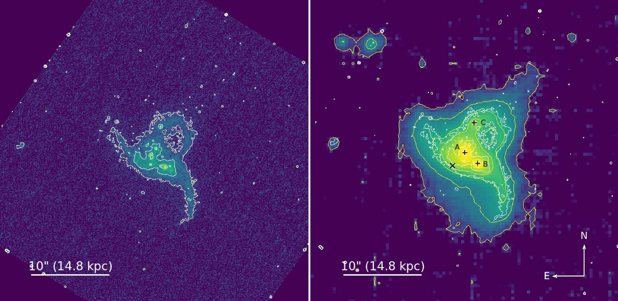
The authors of this study have found signatures of complex organic molecules in protostars forming in the LMC. They focus on the protostar ST6 in the LMC, shown in the right image in Figure 1. They used JWST’s Mid-Infrared Instrument to take spectra of the region around ST6.

Large Magellanic Cloud and N158

Figure 1: The LMC (left) and a zoomed-in view of region N158 (right) containing protostar ST6, the focus of this study. In the inset panel of the right picture, contours of carbon monoxide emission are shown. [Sewiło et al. 2025]

Spectroscopic Signatures of Molecules on Dust Grains

The researchers used the Python tool called dEcompositioN of Infrared Ice features using Genetic Modelling Algorithms (ENIIGMA) to fit the spectroscopy. This code compares the spectra to laboratory data of these complex organic molecules at the temperatures we see in the LMC. The authors fit for complex organic molecules they might expect to see, and they detect methanol (CH3OH), acetaldehyde (CH3CHO), ethanol (CH3CH2OH), methyl formate (HCOOCH3), and acetic acid (CH3COOH); of these, acetaldehyde, ethanol, and methyl formate have never before been detected outside of the Milky Way. Interestingly, this is the first time acetic acid has been definitively detected in any astrophysical environment. The spectral contribution from each molecule is shown in Figure 2; all the individual contributions added together make up the observed spectrum.

spectrum of the protostar ST6

Figure 2: Model fits to the spectrum of the protostar ST6 using the code ENIIGMA. Molecules and their fitted emission are given in the legend. [Sewiło et al. 2025]

These detections provide evidence that these complex organic molecules can be produced on the surfaces of dust grains. Further, their detection in the LMC provides evidence that these molecules can be produced in “harsh” environments like the LMC, with lower metal content and harder radiation fields.

When the authors compared the abundances of these ices to other protostars in the Milky Way galaxy, they found that the abundances are slightly lower around the LMC protostar. This may happen because the dust temperatures are generally higher in the LMC due to the higher-energy photons, which affect the chemistry happening on the dust. Some species they found, however, do have similar abundances to the Milky Way protostars, indicating that the harder radiation field of the LMC does not affect how these species form. Finding more complex organic molecules in the Magellanic Clouds will help us understand further how these compounds form on dust grains and how the galactic environment may affect their formation.

Original astrobite edited by Shalini Kurinchi-Vendhan.

About the author, Caroline von Raesfeld:

I’m a third-year PhD student at Northwestern University. My research explores how we can better understand high-redshift galaxy spectra using observations and modeling. In my free time, I love to read, write, and learn about history.

Illustration of two white dwarfs about to merge

Editor’s Note: Astrobites is a graduate-student-run organization that digests astrophysical literature for undergraduate students. As part of the partnership between the AAS and astrobites, we occasionally repost astrobites content here at AAS Nova. We hope you enjoy this post from astrobites; the original can be viewed at astrobites.org.

Title: Fast Radio Bursts from White Dwarf Binary Mergers: Isolated and Triple-Induced Channels
Authors: Cheyanne Shariat et al.
First Author’s Institution: California Institute of Technology
Status: Published in ApJL

The History of Fast Radio Bursts

Since the discovery of the Lorimer Burst in 2007, astronomers have studied fast radio bursts (FRBs) in extreme detail. However, these extragalactic millisecond-duration radio transients have remained an enigma. Like many astrophysical phenomena, their discovery was serendipitous. The most prolific FRB-discovery instrument, CHIME, was not originally built to study them; the acronym stands for “Canadian Hydrogen Intensity Mapping Experiment,” reflecting its original (and ongoing) mission to map the cosmological distribution of hydrogen in the primordial universe. Since its construction, CHIME has discovered several thousand FRBs and even identified a smaller fraction that are known to repeat, some with consistent periods and others that are sporadic and seemingly random. (Check out their live catalog of repeating sources.)

Despite having thousands of sources to study, the only thing we know fairly confidently about FRBs is that many of them are extragalactic, and some others are even at cosmological distances. If we don’t understand how FRBs are produced, how can we know their distance? FRBs display a unique signature in their radio spectra, where higher frequencies arrive at the telescope first and lower frequencies arrive later, delayed by an inverse frequency-squared relationship. In a “dynamic spectrum,” this makes the pulse actually appear like a sweep from high to low frequency that follows the shape of a parabola; for example, the brightest pixels in Figure 1 of this Bite display this sweeping shape. This effect results from the FRB propagating through an ionized plasma with a specific density. Since the FRB is ultimately an electromagnetic wave, this slows down the speed of the FRB as a function of frequency. Measuring this effect, called dispersion, allows us to infer that the FRB signal passed through more plasma than can be accounted for within our own Milky Way galaxy, indicating that the FRB must have originated from much farther away. So far, there is only one example of an FRB from within our own galaxy, which was identified as originating from a magnetar, a highly magnetic pulsar.

FRB Progenitor Candidates

Although we know that most FRBs are located at extragalactic or even cosmological distances, it’s still not clear what objects that can generate them. Since magnetars and other compact objects are often considered reliable progenitors of FRBs, understanding their populations and comparing them with observed FRBs may reveal the origin of FRBs. Candidate FRB progenitor systems are usually divided into “prompt” channels — like the collapse of a star into a magnetar during a core-collapse supernova — and “delayed” channels where the FRB engine is formed on longer timescales, like accretion-induced collapse of white dwarfs or compact-object mergers. Figure 1 displays several of these channels, particularly those considered in today’s article, in which stellar evolution results in the transfer of material from one star to another (accretion-induced collapse) or gravitational radiation allows two objects to inspiral and merge. These events could create highly magnetized white dwarfs or magnetars that may produce FRBs.

different pathways and their associated fractions for producing an FRB candidate

Figure 1: Three different pathways and their associated fractions for producing an FRB candidate. Depending on the mass and composition of the merging objects, an FRB candidate may be produced instead of causing the white dwarf to explode in a Type Ia supernova. These are the systems of interest in today’s article. [Shariat et al. 2026]

Simulating Hierarchical Triples

In today’s article, we’re considering the role of hierarchical triple star systems in producing FRB-emitting objects. A hierarchical triple consists of an inner binary and a distant, tertiary star; see the first panel of Figure 1. These systems may play an important role because many stars that become white dwarfs of at least 0.8 solar mass exist in hierarchical triples: 35% of 2-solar-mass stars and 50% of 8-solar-mass stars are in triples. Stars of both masses will end their lives as white dwarfs.

The tertiary star plays an essential role in increasing the likelihood of the inner binary interacting: the eccentric Kozai–Lidov (EKL) mechanism causes the inner orbit to oscillate between highly inclined (with respect to the orbit of the tertiary star) and highly eccentric. Unlike isolated binaries that aren’t excited in this way, the eccentric orbit phase causes the inner stars to pass much closer to each other, increasing the likelihood of interaction or even a merger that could produce an FRB-emitting remnant.

The authors of today’s article produced a realistic population of triple systems by sampling from empirically measured distributions of masses, periods, and orbital eccentricities. These distributions were derived from observations collected by the Gaia satellite, an all-sky optical telescope that has now observed more than one billion stars in the Milky Way. The authors also created a “control” sample of isolated binaries by removing the tertiary star from the same sample of systems. The systems were then evolved for an age randomly selected between 0 and 12.5 billion years to simulate “constant” star formation similar to that in the Milky Way. Finally, they reapply these simulations at three different “metallicities” — the fraction of elements other than hydrogen or helium relative to that of the Sun.

Figure 2 displays these two populations: the isolated binaries are shown as filled histograms, and the hierarchical triples are shown as histograms with dashed lines. Each column represents the three different progenitor classes considered in Figure 1. At solar metallicity, the delays to merging are greater in triples than in secular binaries, leading to more mergers overall (top left panel). At lower metallicities, there are fewer mergers in all progenitor pathways in triples than in isolated binaries due to changes in stellar evolution attributed to weaker winds and larger pre-white dwarf masses.

mergers as a function of time for different metallicities and formation pathways

Figure 2: The number of mergers as a function of time from the hierarchical triple’s formation, given different three metallicities (rows) and the three primary formation pathways for FRB-emitting merged remnants considered in Figure 1. Filled histograms are isolated binaries, dashed histograms are triples. [Shariat et al. 2026]

A Cosmic Population of FRBs

Since we can’t realistically track individual star systems from their formation to the end, we need to convert the delay-time distributions shown in Figure 2 to an observable. To do this, the authors combine the results of their simulations with measurements of the cosmic star formation rate — how many stars form per unit time as a function of the universe’s age — and the evolution of the universe’s metallicity as stars fuse hydrogen into heavier elements and return this material to the interstellar medium as these stars end their lives in shedding red giants or supernovae. This analysis produces the number of FRBs that should be observed as a function of distance or lookback time into the universe’s history, which is displayed in Figure 3.

number of FRBs expected as a function of cosmological redshift

Figure 3: The number of FRBs expected as a function of cosmological redshift. The present is to the left, the distant and early universe is on the right. The top panel shows the three formation channels, with binary and triple systems separated. The bottom panel displays the composite rate and compares it with empirical estimates from existing FRB observations. [Shariat et al. 2026]

This analysis reveals key measurable differences between lone binaries and hierarchical triples: most notably, binary white dwarf mergers peak later in the universe (redshift of z ~ 1), while single binaries peak earlier (redshift of z ~ 2). These results highlight the importance of including triples in FRB progenitors because they are more likely to contribute to populations at later times — making them closer and more easily detectable — in the total population of FRBs. Future instruments like CHIME with the new outriggers and the Deep Synoptic Array will expand the sample of FRBs to reach farther cosmological distances, with better localizations, enabling more statistically motivated tests of different formation pathways.

Original astrobite edited by Catherine Slaughter.

About the author, Will Golay:

I am a graduate student in the Department of Astronomy at Harvard University and the Center for Astrophysics | Harvard & Smithsonian, advised by Edo Berger. I study radio emission from transient astrophysical objects like tidal disruption events.

G272.2-3.2

Editor’s Note: Astrobites is a graduate-student-run organization that digests astrophysical literature for undergraduate students. As part of the partnership between the AAS and astrobites, we occasionally repost astrobites content here at AAS Nova. We hope you enjoy this post from astrobites; the original can be viewed at astrobites.org.

Title: Supernova Ia Remnants with M-Dwarf Surviving Companions
Authors: Kuo-Chuan Pan (潘國全), Pilar Ruiz-Lapuente, and Jonay I. González Hernández
First Author’s Institution: National Tsing Hua University
Status: Published in ApJ

Type Ia supernovae are important tools astronomers use to measure distances in space. Despite their important role as “standardizable candles,” their origins remain hotly debated. It’s long been theorized that a Type Ia supernova can develop from one of two pathways: the single-degenerate channel or the double-degenerate channel. In the single-degenerate channel, a white dwarf and a non-degenerate star (such as a red giant or main-sequence star like our Sun) orbit each other in a close binary system. The white dwarf accretes material from the outer surface of the non-degenerate star until it reaches a critical mass and explodes. The double-degenerate channel begins instead with two white dwarfs orbiting each other. Most explosion mechanisms from this channel result in the complete obliteration of the secondary, less-massive white dwarf. However, one theoretical explosion mechanism, called the dynamically driven double-degenerate double-detonation (D6) channel, might allow the secondary companion star to survive an explosion from a double-degenerate Type Ia supernova.

Generally, due to the immense energy from a supernova explosion, we expect these surviving companion stars to be “kicked” away from the blasts at high velocities. Fortunately, astronomers have found evidence of these surviving companion stars. As covered in a previous Astrobite, three hypervelocity white dwarfs have been found in Gaia data and traced back to the locations of double-degenerate Type Ia supernovae. Given the prevalence of Type Ia supernovae, however, astronomers are led to question why we haven’t seen many more of these candidates. It’s additionally important to wonder what similar “runaway” companions might look like for the single-degenerate channel.

Recent observations by the Gaia spacecraft near the supernova remnant G272.2-3.2 show an M-dwarf star, MV-G272, with an unusually high velocity around 240 km/s and a trajectory tracing back to the center of the supernova remnant. Is it possible for this M dwarf to be the runaway companion to the remnant’s original supernova? The authors of today’s article look at simulations of potential companion stars from single-degenerate Type Ia supernovae and compare their results to this observed potential companion candidate.

Because this work focuses on the potential for M-dwarf companions, the authors explored a range of simulated companion-star masses and radii characteristic of M dwarfs: 0.5, 0.6, and 0.7 solar mass and 0.396, 0.454, and 0.483 solar radius, respectively. To make these models, they used the stellar evolution code Modules for Experiments in Stellar Astrophysics (MESA) to construct and evolve a number of simulated stars with these specifications.

After setting up the models in MESA, they used the magnetohydrodynamics code FLASH to perform 2D and 3D simulations of the supernova explosion and the subsequent impact of the exploding star’s ejecta (or hot material) on its M-dwarf companion. After the explosion and impact were modeled, the companion star’s evolution was further followed in MESA.

Figure 1 shows the density of the supernova’s ejecta, or exploding material, as it impacts the companion star. (You can think of this figure as if you were looking at the companion star out in space.) After roughly 100 seconds, you can see a bow shock develop around the top of the companion (or the “front” of the star) as it wraps around the companion. This impact causes significant compression of the companion star and rips away upwards of 50% the companion’s mass. The impact of this shock is what gives the companion star its “kick,” sending it hurtling through space.

simulations of supernova ejecta colliding with a star

Figure 1: Visual of the density of the companion star (center of each plot) and the supernova ejecta over time. In the top row of plots and the bottom-left plot, you can see the higher-density bow shock bent around the top (or front) of the companion star. In the bottom-right plot, you can see some of the supernova ejecta and unbound mass from the companion star settling around the companion star. [Pan et al. 2025]

Because the authors explored a range of initial companion masses and distances between the primary and companion star, their results show some range. Figure 2 shows two important results: the evolution of the companion’s mass before and after the explosion (left plot), and the evolution of the companion’s kick velocity (right plot). The dip in mass around 100 seconds (102 s) indicates the impact of the bow shock. Even though the simulations model companions with a relatively narrow mass range (0.3–0.7 solar mass), there is considerable variation in the final masses after explosion. For example, the initial 0.5-solar-mass model ends up with anywhere between 0.07 solar mass (just 14% of its initial mass) and almost its full initial mass of 0.5 solar mass, depending on the distance between the companion and its exploding star.

plots of bound mass and kick velocity as a function of time

Figure 2: The different models shown in both plots indicate different initial masses and separation distances between the companion and the exploding star. Left: how the companion’s gravitationally bound mass evolves over time. The plot can be read left to right. The dip around 102 seconds indicates the impact of the supernova shock, which unbinds layers of the companion’s mass. Some of that mass becomes bound again to the companion after the shock passes. Right: how the companion star’s kick velocity changes based on initial mass and separation distance between companion and exploding star. The peak in values between 102 and 103 seconds indicates the impact, or “kick,” from the supernova. [Pan et al. 2025]

The results from this work generally show, predictably, that a companion closer to its primary star gets a bigger kick in velocity. These “kicks” range from about 50 km/s to 150 km/s. When added to the system’s initial velocity in space, it brings the total velocity of these companions into the 150–200 km/s range. This result is generally well aligned with the observed velocity of MV-G272, which was roughly 240 km/s.

Notably, runaway companion stars of these Type Ia supernovae seem to retain information from the initial explosion. Given the final velocities of these companions, astronomers might be able to figure out the companion’s initial mass and trace back its trajectory to the system it originated from. Overall, the fact that MV-G272 has a trajectory that tracks back to the center of a supernova remnant makes it a good companion candidate. These results support the feasibility of M-dwarf runaway companions from single-degenerate Type Ia supernova systems. Now that we know what these companions might look like — and how fast they can be going — astronomers can hopefully better search for these high-velocity stars in the future.

Original astrobite edited by Catherine Slaughter.

About the author, Mckenzie Ferrari:

I’m currently a PhD student in the geophysical sciences program at the University of Chicago. While I now study the atmosphere and oceans of Earth, most of my previous research focused on simulations of Type Ia supernovae and galaxy formation and evolution. In my free time, I foster cats for a local organization, enjoy cooking, and can often be found running along Lake Michigan.

illustration of an accreting black hole

Editor’s Note: Astrobites is a graduate-student-run organization that digests astrophysical literature for undergraduate students. As part of the partnership between the AAS and astrobites, we occasionally repost astrobites content here at AAS Nova. We hope you enjoy this post from astrobites; the original can be viewed at astrobites.org.

Title: The z = 7.08 quasar ULAS J1120+0641 May Never Reach a “Normal” Black Hole to Stellar Mass Ratio
Authors: Meredith A. Stone et al.
First Author’s Institution: University of Arizona
Status: Published in ApJ

The first galaxies in the universe emerged out of an archaic age of darkness. Like luminous factories, they started rapidly churning out stars, spilling light into the cosmos. This process of star formation continues to the present day. In some galaxies, it occurred at astonishing rates, with the equivalent of thousands of times the mass of the Sun being assembled into stars in a single year. At other times, it came to a slow crawl, with all fresh reserves of star-building gas seemingly exhausted. Yet when the gears of star formation ground to a halt, certain events were able to send them spinning again.

One of the most spectacular of these is a merger, a train-wreck collision between two galaxies. Images of these events are often breathtaking, showing arms of light twisting together and vast stellar streams being violently cast away. Mergers directly increase the stellar mass (the mass of all stars) of galaxies by combining two into one. The intense gravitational interactions between the galaxies involved can also disrupt stagnant pools of gas, igniting a new burst of star formation. Thus, interactions between galaxies can be a significant driver of their growth.

Sometimes, a reservoir of matter is driven toward the center of a galaxy due to a “secular” process (one that occurs without external intervention) or from a merger. At the galactic nucleus, the infalling streams of matter encounter a supermassive black hole. The matter falls into a swirling accretion disk, heating to extreme temperatures and furiously glowing. If the black hole is massive enough and the gas falls in quickly enough, the accretion disk can outshine all of the stars in the galaxy, and we call such a source a quasar. The intense radiation produced by a quasar can impact the entire rest of the galaxy, either suppressing the formation of new stars or sometimes igniting it.

Thus, a galaxy has an important role in the growth of its central supermassive black hole, and vice versa. This connection manifests in complicated ways. Most strikingly, it is thought to be the cause of the correlation between a galaxy’s stellar mass and its central black hole mass. In the nearby universe, galaxies have stellar masses around a thousand times greater than their black hole masses. JWST, our most powerful tool for investigating early galaxies, has given us unprecedented insight into whether this holds up in the distant universe. Though the jury is still out, many researchers are convinced that the answer is a resounding no. We’ve found distant black holes that appear to be nearly equal in mass to their host galaxies, something that’s unfathomable in the local universe.

However, this raises a key question. Black holes and their galaxies grow together, and they started on nearly equal footing. So why do all of the galaxies in the nearby universe appear so much more massive than their black holes? Today’s article underscores this puzzle, pushing it to the breaking point. The authors examine a well-studied quasar, ULAS J1120+0641 (hereafter J1120), which we see as it appeared just 750 million years after the Big Bang. This source has a supermassive black hole containing an astounding 20% the mass of its host galaxy. The shocking part is that, even after carefully accounting for all of the ways this galaxy could grow in the future, there appears to be no way for J1120 ever to reach “normal” proportions.

Through the Looking Glass, ULAS J1120

First, the authors analyze the key observations of J1120 obtained to date. In addition to observations from JWST, this source has been targeted by some of the most powerful astronomical facilities, including the Hubble Space Telescope (optical and near-ultraviolet), the Chandra and XMM-Newton observatories (X-rays), the Atacama Large Millimeter/submillimeter Array (radio/millimeter), and numerous other ground-based telescopes. This incredible dataset provides a detailed picture of J1120 across the electromagnetic spectrum, spanning X-rays to radio emission.

The authors compare various measurements of the black hole’s mass and find that multiple methods yield a similar result of about a billion and a half times the mass of the Sun. Turning to the host galaxy, they estimate the mass of the visible stars, which is more complicated than it sounds — you can’t exactly count them, since the enormous distance between us and J1120 causes it to appear as just a fuzzy blob. They combine this mass with the mass of newly forming stars that are buried in dust and obscured from our view. The mass of a nearby galaxy that’s actively merging with J1120 is added to this sum. Finally, the authors compute how many stars could form in the future from all of the gas left in the galaxy, and they throw this into the total.

Even with all of these components, the host galaxy would only be 10 times more massive than the black hole at the center. This ratio is a far cry from the factor of a thousand we expect for normal galaxies in the local universe!

A Train Wreck of Train Wrecks

Well, if one merging galaxy won’t do it, what if J1120 merges with literally every single other nearby galaxy? The authors use new JWST data to count all sources near the quasar (Figure 1) and measure their stellar masses. Going further, they estimate how many galaxies their technique may have missed and add all of these to the pile. Not done yet, they finally conclude by making a rough approximation of how much loose gas is in these nearby galaxies, and compute how much extra mass could exist in stars born from this fresh material. Assuming that J1120 survives the full-frontal assault, being battered by mergers from each of its neighbors in turn, its total stellar mass would grow by quite a large factor.

J1120 and nearby galaxies

Figure 1: All of the galaxies found by JWST that are close enough to J1120 to potentially merge with it in the future. The circles mark confident detections, whereas the squares represent galaxies for which the exact distances couldn’t be measured confidently. What would happen if all of these galaxies crashed into J1120? [Stone et al. 2025]

What’s the final result? Shockingly, even after all of this growth, the stellar mass of J1120 would still only be about 40 times that of the central black hole. That’s 25 times less than we’d expect from a nearby galaxy! Even if the black hole never grows again, it appears that this galaxy will never reach “normal” proportions. So why is it that, when we look around at the local universe, there’s nothing like J1120? The authors point out that galaxies near J1120 would be missed by their methods if they are obscured by thick shrouds of gas and dust. Such sources would increase the estimated mass that could be contributed by mergers. On the other hand, maybe J1120 will adopt the strategy of the blue whale, filter feeding on the extremely sparse matter between galaxies, yet growing to enormous proportions.

A fascinating final possibility is that galaxies like this one do exist in the nearby universe. With their black hole switched off, all we would be able to see is a relatively small package of stars. Place such an object far enough away, and we might miss it entirely! Whether galaxies like J1120 achieved normal proportions through unknown mechanisms or are lurking in the far fringes of the local universe, studies like this one shine light on the amazing connection between black holes and their host galaxies. In the future, they will be one key piece in the puzzle of the endlessly complicated past of our own galaxy and the universe at large.

Original astrobite edited by Will Golay.

About the author, Ansh Gupta:

I’m an astronomy graduate student at the University of Texas at Austin working with Steven Finkelstein. I use data from JWST to study the formation and growth of the first galaxies and black holes in the universe. In my spare time, I enjoy playing piano, reading, and making YouTube videos.

NGC 3603

Editor’s Note: Astrobites is a graduate-student-run organization that digests astrophysical literature for undergraduate students. As part of the partnership between the AAS and astrobites, we occasionally repost astrobites content here at AAS Nova. We hope you enjoy this post from astrobites; the original can be viewed at astrobites.org.

Title: Characterizing The Star Cluster Populations in Stephan’s Quintet Using HST and JWST Observations
Authors: P. Aromal et al.
First Author’s Institution: University of Western Ontario
Status: Published in ApJ

On 12 July 2022, the first images taken with JWST were released to the public. All of the astronomers in my department gathered together to watch the images be revealed in real time. It was exciting for everyone, from graduate students getting to see a glimpse into the future possibilities of their fields, to retired professors getting to see the fruits of their decades-long labor in advocating for the telescope to be built.

One image that was showcased was of Stephan’s Quintet (Figure 1), an actively interacting galaxy group. We were all immediately impressed by the clarity of the star-forming regions in the dense gas between the galaxies in the image. Now, more than three years later, the authors of today’s article lay out a comprehensive study of the star clusters in those same regions, taking advantage of JWST’s multi-wavelength imaging capabilities.

Stephan's Quintet

Figure 1: The JWST imaging of Stephan’s Quintet with member galaxies labeled (including NGC 7320C, which is outside of the field of view). Gray arrows indicate the direction the associated galaxy is moving. The inlaid image shows the distribution of young star clusters in relation to the six main tidal features in the group. [Inset image: Adapted from Aromal et al. 2025; Background image: NASA, ESA, CSA, STScI]

HST + JWST = OMG!

While JWST’s depth and resolution are exciting for those studying high-redshift galaxies, for local-universe astronomers JWST really shines when used in combination with the Hubble Space Telescope (HST). The star clusters in Stephan’s Quintet were already cataloged in 2015 using HST, but the filters used in the imaging only captured optical and very-near-infrared wavelengths. If you want to get enough data to be able to accurately estimate the ages of these star clusters, especially accounting for reddening caused by surrounding dust, you need to push your imaging further into the infrared.

Unlike HST, JWST can take images in two wavelength filters at once, meaning you can get more data with roughly the same observing time. Here the authors imaged the same star clusters that HST looked at with five new JWST filters, all at longer infrared wavelengths than HST. Together, the authors had flux measurements at 10 different wavelengths across the optical and infrared spectrum for each star cluster, meaning they could perform spectral energy distribution fitting.

Go Ahead, Guess My Age

The best way to estimate an unresolved star cluster’s age is to get its full spectrum of light and fit spectroscopic models with varying ages to it until the model matches the observations. But, if you have individual brightness measurements at many different, spread-out wavelengths, you can still fit spectral models to the measurements and make a best guess despite the gaps in your full spectrum. Here the authors compare their multi-wavelength data to Code Investigating GALaxy Emission (CIGALE) spectral energy distribution models, allowing both the cluster ages and amount of dust extinction to vary.

This is where the long-wavelength JWST imaging is most necessary, because it is sometimes difficult to determine a cluster’s age with this method. For instance, is the light a cluster is giving off mostly red because its stars are very old, or is it because its stars are actually bluer and younger and the cluster just appears red due to foreground dust?

Infrared imaging can “see through” any dust and break this age–extinction degeneracy. For most of the clusters, the authors found that the original HST-only age estimates were accurate, but for 121 clusters in the sample (about 8% of the total), the JWST imaging made a significant change in the age estimates, shifting them to younger ages.

Where Do the Hip, Young Star Clusters Hang Out?

Once the authors had their updated ages for the clusters, they then mapped out where the clusters were located in Stephan’s Quintet and how these clusters traced the known tidal structures in the group. Tidal structures are structures, usually consisting of gas, dust, and stars, that are formed from the tidal forces galaxies exert on one another as they interact and merge. The authors found that throughout all tidal regions of Stephan’s Quintet, there were many young, low-mass star clusters, all about 3–5 million years old. This timescale lines up with previous studies’ estimates of when NGC 7318B was thought to first fall into Stephan’s Quintet, compressing the gas in the group and creating tidal shocks that would trigger star formation.

Additionally, the authors’ star cluster age distribution for the group (see Figure 2) has a second, broader peak of higher-mass clusters with ages around 200 million years. This would correspond to when the most recent encounter between NGC 7320C (which has now passed through the group and is out of frame in Figure 1) and NGC 7319 is estimated to have occurred.

histogram of the ages of all the star clusters in Stephan's Quintet

Figure 2: A histogram of the ages of all the star clusters in Stephan’s Quintet. The blue dashed line shows the estimates using only the HST data, and the orange solid line shows the estimates using both HST and JWST together. Notice how a lot of the clusters around 108 years old turned out to be less than 107 years old. [Adapted from Aromal et al. 2025]

Going even older, they found that the star clusters in the group that are more than 1 billion years old are also the most massive, and they are predominantly concentrated around NGC 7318A. This is the most massive elliptical galaxy in the group, and it’s the most likely to have a rich, old star cluster population, formed prior to any tidal interactions.

Taken together, the updated age measurements of the star clusters in Stephan’s Quintet provide not only a study of star formation history, but also of the galaxy–galaxy interaction history in the system!

Looking Ahead

While the authors have improved the age estimates of the clusters in Stephan’s Quintet, there are still limitations to their analysis. Their estimated star formation rate for the group is much lower than that estimated with other tracers, such as H-alpha emission, meaning this study may still be missing a fraction of very young star clusters. The most likely culprits are embedded clusters that haven’t had enough time to expel the surrounding gas from the massive clouds they formed within.

Future work will attempt to identify these embedded clusters using near-infrared JWST imaging, since in this study the authors focused only on the previously HST-identified clusters. In addition, combining their JWST data with high-resolution radio observations taken with the Atacama Large Millimeter/submillimeter Array will allow them to study the gas in the group more closely and understand how it influences the star formation.

This work highlights JWST’s excellent application to star cluster observations, building on the data we already have from decades of HST use, and it looks like we’re only just getting started!

Original astrobite edited by Skylar Grayson.

About the author, Veronika Dornan:

Veronika is a postdoctoral research associate at the University of Edinburgh. Her research is in observations of globular star clusters and how they can be used to study the evolution of their host galaxies.

G299.2-2.9

Editor’s Note: Astrobites is a graduate-student-run organization that digests astrophysical literature for undergraduate students. As part of the partnership between the AAS and astrobites, we occasionally repost astrobites content here at AAS Nova. We hope you enjoy this post from astrobites; the original can be viewed at astrobites.org.

Title: The First Day of a Type Ia Supernova from a Double-Degenerate Binary
Authors: Gabriel Kumar, Logan J. Prust, and Lars Bildsten
First Author’s Institution: University of California, Santa Barbara
Status: Published in ApJ

Much like distance markers along the highway, Type Ia supernovae have long been used as distance indicators in space. These supernovae were originally theorized to form in binary systems. In this system, a white dwarf (a dense, collapsed remnant of a star) steals surface material from a non-degenerate star like our Sun and then explodes. Because of the initial conditions and properties of those two stars, the explosion would shine with the same intrinsic brightness regardless of the binary system’s location in space.

Research and observations, however, show that this is not entirely true; not all Type Ia supernovae are equally luminous. There are various theories regarding the different formation scenarios and explosion mechanisms that might create a Type Ia supernova. Developing ways to sleuth out the origins of these systems can be useful because it may tell us more about their luminosity.

One emerging theory of formation is the “double-detonation scenario.” In this case, two white dwarfs exist in a binary system. The more massive primary (the “accretor”) steals material from the less massive white dwarf secondary (the “donor”). After the primary steals the donor’s outer thin shell of helium, the helium surrounding the accretor detonates. This explosion induces a shock wave that travels into the dense core of the accretor and causes another detonation. The two detonations — one on the surface and one in the core — produce enough energy to explode the star into a supernova, a powerful stellar explosion. When the material from the exploding star reaches its companion star, it forms a mysterious, conical wake within the gaseous material, or “ejecta,” expelled from the accretor. This wake might be an important clue for distinguishing a supernova’s origins.

Since these explosions are incredibly powerful and would be difficult (and dangerous!) to perform in a lab, astronomers turn to computer simulations to model these events. Hydrodynamical simulations, in particular, are helpful for researchers because they model how fluids “flow” by solving complex equations that are too tricky to do by hand. (Remember that stars are just balls of gas, and hence fluid!) The authors of today’s article ran hydrodynamical simulations of the explosion and subsequent evolution of the ejecta from a double-detonation scenario.

In the diagram of the team’s setup (see Fig. 1), you can see a “bow shock.” This shock is from the wave produced in the accretor’s detonation and is bowed since it bends around the donor star. This shock moves quickly through the cone of ejecta, modifies its structure, and leaves clues within the ejecta as it settles.

schematic of the simulation setup

Figure 1: A visual schematic of the simulation setup. The accretor is the exploding star, which produces a “bow shock” from the detonation. The bow shock and recompression shock modify the structure of the ejecta, which fills the space between rout and rin. The ejecta is full of gaseous stellar material. [Kumar et al. 2025]

After simulating 1,000 seconds after the explosion, the authors recreated a high-density, low-temperature “wake” from the shock. You can see imprints of this wake in Fig. 2, as denoted by the red arrow.

visual slice of the simulated ejecta

Figure 2: A visual “slice” of the ejecta surrounding the donor star just 200 seconds after detonation. The bottom-left corner (r = 0) has a faint white spot, indicating the donor. The density (top) and temperature (bottom) of the ejecta are shown. The faint line marked by the red arrow indicates the secondary shock from the explosion, highlighting changes in both density and pressure. [Kumar et al. 2025]

Once they were able to produce this wake, the authors evolved the ejecta over time to see what the radiation from this material might reveal. They discovered that the “shocked,” or compressed and heated, ejecta flew out much further than the unshocked ejecta (see Fig. 3).

simulation snapshot at 2 hours of simulation time

Figure 3: A slice of the simulation taken later, at 2 hours of simulation time. The ejecta in the shocked region has flown out farther than the ejecta in the unshocked region. Note that the horizontal scale has changed from Figure 2. [Kumar et al. 2025]

This ejecta can be seen from different viewing angles, influencing an observer’s measurement of the explosion’s luminosity. The strongest features of the wake are visible up to about 55 degrees, while some effects can still be seen up to about 140 degrees — almost half of the sky (see Fig. 4). Overall, an observer’s position relative to the explosion axis might change their reported luminosity of the explosion. The authors estimate that this wake might cause Type Ia supernovae from a “double-detonation” scenario to appear up to 15% fainter, depending on the observer’s viewing angle. Therefore, if scientists use Type Ia supernovae as cosmic distance indicators, their calibrations might be slightly off. This isn’t the best news for those using measurements of Type Ia supernovae to measure the expansion rate of the universe.

plot of luminosity versus time after detonation of a supernova

Figure 4: A comparison of luminosity vs. time over the course of 6 hours shortly after detonation. The different lines indicate different viewing angles from the axis of explosion. The line “Analytics” describes a light-curve prediction by Piro (2012) for a supernova that was not shock-heated. The luminosities for this model span almost one order of magnitude. [Kumar et al. 2025]

We’ve talked a lot about the accretor and ejecta in this scenario, but what might happen to the donor star? One idea is that the donor star is “kicked” away by the high velocity of the blast. In this simulation, the authors were able to calculate a “kick” velocity, or speed imparted by the blast to the donor star, that was much higher than estimates from other detonation models. One observed Type Ia supernova, SN 2021aefx, is believed to have the fastest observed ejecta to date. The mechanism that today’s authors modeled might explain how the ejecta of this event got its super-fast “kick.”

While there is always more work to be done, this work presents a first step at identifying double-detonation Type Ia supernovae from early observations. With an influx of observations from new observatories, like the Vera C. Rubin Observatory, we should expect to see many more early supernova detections.

Original astrobite edited by Ansh Gupta.

About the author, Mckenzie Ferrari:

I’m currently a PhD student in the geophysical sciences program at the University of Chicago. While I now study the atmosphere and oceans of Earth, most of my previous research focused on simulations of Type Ia supernovae and galaxy formation and evolution. In my free time, I foster cats for a local organization, enjoy cooking, and can often be found running along Lake Michigan.

SDSS J0849+1114

Editor’s Note: Astrobites is a graduate-student-run organization that digests astrophysical literature for undergraduate students. As part of the partnership between the AAS and astrobites, we occasionally repost astrobites content here at AAS Nova. We hope you enjoy this post from astrobites; the original can be viewed at astrobites.org.

Title: Episodic Feedback in Triple Active Galactic Nucleus Candidate SDSS J0849+1114 Revealed by Extended Ionized Gas
Authors: Xiaoyu Xu (许啸宇) et al.
First Author’s Institution: Nanjing University
Status: Published in ApJ

When Galaxies Collide

Galaxies are social creatures; they interact and merge (more astrobites talking about this are here and here)! When galaxies collide, the gravitational chaos acts like a funnel, driving massive amounts of cold gas toward the center. This gas rush has two major consequences: it triggers intense bursts of star formation (known as starbursts), and it feeds the central supermassive black holes, activating them as active galactic nuclei (AGNs).

But the story doesn’t end there. These powerful AGNs don’t just sit and feast on the gas. They launch high-velocity winds or jets that push back against the incoming gas, a process known as AGN feedback. (Read more about it in Astrobites here and here.) This feedback is thought to be the key mechanism by which supermassive black holes regulate their host galaxies, either by heating and expelling the gas (negative feedback, which starves star formation) or, in some cases, by compressing it (positive feedback, which promotes star formation).

While binary AGNs (two AGNs in one merging system) are rare, finding systems with three AGNs in one system is fascinatingly rare. The galaxy SDSS J0849+1114 (J0849+1114) is one such system, featuring three Seyfert 2 AGNs, a type of active galaxy with a bright, compact nucleus whose spectrum shows only narrow emission lines, within a tight region of about 5 kiloparsecs (kpc) or 16,000 light-years. Studying this system gives us a front-row seat to how multiple black holes interact and regulate their host environment during a complex merger. Very Large Array observations reveal that nucleus A (see Figure 1) contains two jets, inner and outer. In contrast, nucleus C has one jet, providing further evidence for the presence of an AGN.

Hubble and Very Large Telescope images of J0849+1114

Figure 1: Left: Hubble Space Telescope image taken in ultraviolet light. Right: Optical image from the VLT/MUSE instrument. The three black holes, nuclei A, B, and C, are marked with black crosses. The white contours are from Hubble, like on the left, and the yellow contours are of the MUSE instrument. We can observe the complex and disturbed morphology resulting from the ongoing merger. [Adapted from Xu et al. 2025]

Peering into the Triple Core with VLT/MUSE

To understand the gas dynamics in J0849+1114, the authors used the Very Large Telescope (VLT) and its Multi-Unit Spectroscopic Explorer (MUSE) instrument. MUSE is an integral-field spectrograph, meaning it provides spectra for every single spatial pixel (or “spaxel”) across the field of view. This allows astronomers to map not just where the light is coming from, but how the gas is moving and what is causing it to glow, all resolved spatially across the galaxy.

The main technique employed was two-component Gaussian fitting of key emission lines like hydrogen alpha (Hα) and ionized oxygen ([O III]λλ4959,5007), which can be seen in Figure 2. The width of a Gaussian line (or its velocity dispersion) in a spectrum tells us how fast the gas is moving. A narrow line means the gas is relatively calm, with most of it moving at similar speeds. A broader line, on the other hand, means the gas velocities are more spread out — some parts are racing toward us, others away — indicating turbulence or outflows. By comparing the widths of different components, astronomers can separate quiet, rotating gas from the high-speed winds launched by the active black holes.

spectra of J0849+1114

Figure 2: Zoomed-in spectra showing the Hβ and [O III] (left) and Hα, [N II], and [S II] (right) emission lines from the spot marked with an “X” in the MUSE image in Figure 1. The blue line shows the observed data, the orange line shows the best-fit model, and the two colored curves (light blue and red) represent the two components of the gas. The pink line shows the leftover differences between the data and the model. The First Component is narrow, representing gas that is relatively settled, often showing signs of rotation or slow movements associated with gravitational disturbances, like tidal tails (low velocity dispersion, σ1 ≤ 50 km/s). The Second Component is broad, representing highly turbulent or fast-moving gas, characteristic of powerful outflows or winds driven by the central AGNs (high velocity dispersion, σ2 > σ1). [Adapted from Xu et al. 2025]

What They Found: Gas Tails and Outflows

The VLT/MUSE observations successfully characterized both the undisturbed (First Component) and turbulent (Second Component) gas across the system.

1. Galactic-Scale Tidal Tails

The slow-moving gas (First Component) revealed extended structures of ionized gas stretching over 10 kpc (33,000 light-years), and in some directions, even more than 15 kpc (49,000 light-years) away from nucleus A. These large, low-velocity gas clouds align well with features known as tidal tails: the stretched-out arms of gas and stars pulled away by the violent gravitational forces of the merger.

2. Two Distinct Outflows Driven by Radio Jets

The fast-moving gas (Second Component) clearly showed two distinct sites: outflows originating from nucleus A and nucleus C.

  • Outflow A: This outflow extends over 5 kpc (16,000 light-years) around nucleus A. The gas kinematics and geometry strongly suggest that this outflow is being driven by nucleus A’s radio jet. This finding is key, as the measured kinetic power of the outflow is about 10 times stronger than what star formation alone could supply, and the current luminosity of the AGN is also insufficient to power it.
  • Outflow C: A smaller but detectable outflow extends about 5.9 kpc (19,000 light-years) around nucleus C, with a lower kinetic power compared to Outflow A. But, like Outflow A, the energetics and velocity gradients suggest this outflow is also linked to nucleus C’s radio jet.

A Black Hole That’s Recently Gone Quiet

The most striking implication of this study relates to the timing of nucleus A’s activity. The presence of extended ionized gas far from the nucleus (in the tidal tails, >10 kpc or 33,000 light-years away) provides a fascinating glimpse into the AGN’s recent past.

The physical conditions of this distant gas were determined using emission line ratios ([O III]/Hα and [N II]/Hα) on the Baldwin, Phillips, and Terlevich (BPT) diagram. A BPT diagram uses emission line ratios to diagnose the energy source that ionizes the gas: star formation, AGN, or shocks. The BPT diagram of J0849+1114 indicates that an AGN currently photoionizes the gas.

By running sophisticated photoionization models, the scientists calculated how luminous nucleus A must have been to ionize the gas currently found 10–15 kpc (33,000–49,000 light-years) away. They discovered that this required nucleus A to be 20–100 times more luminous than it currently is! Since light takes time to travel, and the ionized gas quickly recombines (on timescales of less than 100 years for this gas), this luminous phase must have ended very recently, approximately 30,000–50,000 years ago. This is a long time for us, but just a blink of an eye on cosmic timescales.

The Episode of Self-Regulation

By integrating the findings across different wavelengths and timescales, the current faint luminosity state, the past luminous state inferred from the distant gas, and the presence of radio jets of different ages, the authors propose a model of episodic AGN feedback in nucleus A:

  1. Past Activity (150,000 years ago): An active phase likely launched an outer radio jet, which subsequently drove the large-scale ionized gas outflow observed today.
  2. Peak Ionization (30,000–50,000 years ago): A subsequent burst of high accretion reached its peak, ionizing the distant tidal tails.
  3. Fading and Quenching (Today): The energy released by the jet and/or outflow during the active phase likely expelled or heated the surrounding gas (negative feedback), causing the central accretion disk to run out of fuel. The AGN has since faded rapidly to its current low-accretion state, marked by the appearance of a young inner radio jet.

A Quiet Ending After a Loud Beginning

J0849+1114 is not just a statistical anomaly as a triple AGN candidate; it serves as a crucial case study demonstrating the powerful and rapid effects of AGN feedback. High-resolution observations confirm that violent galaxy mergers trigger both powerful outflows and episodic bursts of extreme luminosity. Crucially, these outflows clear the gas and cause the central supermassive black hole to quickly fade from a luminous quasar phase to a quiet, low-accretion state within tens of thousands of years. This system provides strong, spatially resolved evidence that AGN feedback rapidly suppresses accretion onto the supermassive black hole and shapes the host galaxy on kiloparsec scales during the chaotic drama of galactic mergers.

Original astrobite edited by Lindsey Gordon.

About the author, Sowkhya Shanbhog:

I am currently a first-year PhD student at Scuola Normale Superiore in Pisa, Italy, where I am focusing on studying high-redshift quasars. Prior to this, I completed a dual BS-MS degree at the Indian Institute of Science Education and Research in Pune, India. Now, I am eager to expand my involvement in science communication and outreach initiatives. I have recently developed an interest in cooking, particularly since moving to a new city. I find solace in listening to music during my leisure time.

illustration of a planet getting uncomfortably warm

Editor’s Note: Astrobites is a graduate-student-run organization that digests astrophysical literature for undergraduate students. As part of the partnership between the AAS and astrobites, we occasionally repost astrobites content here at AAS Nova. We hope you enjoy this post from astrobites; the original can be viewed at astrobites.org.

Title: Near the Runaway: The Climate and Habitability of Teegarden’s Star b
Authors: Ryan Boukrouche, Rodrigo Caballero, and Neil T. Lewis
First Author’s Institution: Stockholm University
Status: Published in ApJL

To find life on other planets, we start our search for planets like Earth. (It’s the best example of a habitable planet that we know of!) Earth’s distance from the Sun allows for liquid water to exist on the surface, which is vital for life as we know it. This region, called the “habitable zone,” describes the right atmospheric conditions and proximity to its host star that a planet can have to support liquid water. Earth is also special because of its atmosphere, which contains greenhouse gases such as water vapor and carbon dioxide (CO2); these help keep the average global temperature moderate enough for life to exist.

A few factors govern the habitable zone for a given planetary system: for example, the strength of a star’s radiation, the composition of the planet’s atmosphere, and a planet’s orbital period around its star. This is because a planet’s “energy budget” is dictated by these factors. For a planet to have a “stable” climate, the energy it receives from its star must balance the energy it re-emits. For instance, in a given planetary system, the closer a planet’s orbit is to its host star, the more sunlight it receives and therefore the more energy it must radiate away. This balance is between outgoing longwave radiation, which is heat emitted by the planet, and absorbed/incoming shortwave radiation, which is the sunlight the planet receives from its host star.

Some Earth-like analog planets have piqued the interest of astronomers because observations suggest that they lie within the habitable zones of their respective stars. One system, named after its discoverer, Bonnard Teegarden, features an M-dwarf star with three orbiting Earth-mass planets. It exists about 12.5 light-years away, making it one of the closest planetary systems to us. One of the planets, Teegarden’s Star b, is believed to have very similar characteristics to Earth: a radius of 1.02 REarth and a mass of 1.16 MEarth. Because the planet orbits an M-dwarf star, which is much cooler (temperature-wise) and less massive than our Sun, the planet’s orbit is much, much smaller than Earth’s, with a semimajor axis of 0.0259 au (compared to 1 au for Earth) and an orbital period of 4.9 days (compared to 365 days for Earth).

The authors of today’s article explore how close Teegarden’s Star b is to its habitable zone based on current observations, and how future observations could lead to vastly different interpretations of its habitability.

Exoplanets are small and faint, making it difficult for current technology to study their atmospheres accurately. Modern simulations, known as general circulation models, can model how a planet’s atmosphere might behave under various assumptions. Isca, the climate and atmospheric dynamics model used in this article, has been used to model exoplanetary atmospheres in previous studies. Modeling a planet around an M-dwarf, the authors tried matching the planet’s properties as closely as possible to Earth, using a simple cloud model (which is challenging to model), moist physics (since our atmosphere contains water vapor), and a radiative transfer scheme. In their simulation, the authors also assumed that Teegarden’s Star b is tidally locked, meaning its dayside always faces its sun. For example, our Moon always shows the same side to us on Earth and is considered tidally locked.

They also assigned Teegarden’s Star b a similar atmospheric composition to Earth: 78% nitrogen (N2), 28% oxygen (O2), and a CO2 concentration of 400 parts per million by volume (ppmv). Unlike Earth, they did not include an ozone layer; however, they state that including one did not significantly change the results. Combinations of these different factors were run for 8–41 Earth years, until the Teegarden’s Star b model either reached a stable state (where the energy balance equals 0 W/m²), or it exceeded the runaway greenhouse gas threshold — the point at which the energy balance exceeds zero, and the planet’s surface temperature increases uncontrollably.

The average amount of radiation that a planet receives is called its instellation, or sometimes “insolation” when talking about our Sun. For reference, Earth has an insolation value of around 1365 W/m². Different studies of Teegarden’s Star b suggest an instellation of 1481 W/m² or 1565 W/m², so the authors multiple values in that range (see Fig. 1).

plots of modeled energy balance over time for Teegarden's Star b

Figure 1: For a surface albedo of 0.07 (ocean-dominated), the energy balance for each tested instellation (ISR; 1481–1540 W/m²) is shown. As time increases, a stable atmosphere would consistently reach an energy imbalance value of 0 W/m². In contrast, an unstable (runaway greenhouse) atmosphere would have a value greater than 0 W/m², indicating that it is receiving more energy than emitting. [Boukrouche et al. 2025]

The biggest difference in results comes from the two different instellation values of 1480 and 1565 W/m² (see Fig. 2). For 1480 W/m², Teegarden’s Star b lies just within the habitable zone, but admittedly not by much. It’s only about 20–40 W/m² away from becoming uninhabitable. This would give Teegarden’s Star b a mean surface temperature about 18K higher than that of present-day Earth. Since a difference of one Kelvin is equivalent to a difference of one degree Celsius, this corresponds to a temperature of 18℃ (32.4℉) above your average day on Earth — pretty hot and unlikely to be comfortable for lifeforms similar to ours. The precipitation would also be similar to the wettest regions of the Sahara Desert, so overall, Teegarden’s Star b would be a relatively dry planet. For 1565 W/m², Teegarden’s Star b crosses the runaway greenhouse threshold and cannot be considered habitable for life similar to ours.

global mean surface temperature and planetary albedo of Teegarden's Star b

Figure 2: The global mean surface temperature (top) and planetary albedo (bottom) of Teegarden’s Star b are shown with various instellation values. The filled markers represent models that reached an equilibrium, or stable, state, whereas the empty markers are models that reached a runaway, uninhabitable state. The two vertical black lines represent the two main instellation estimates of 1481 and 1565 W/m². Once the models exceed the ~1520 W/m² instellation value, they start to fail and reach a runaway greenhouse effect. [Boukrouche et al. 2025]

Our best guess of the habitability of Teegarden’s Star b is highly dependent on future observations and measurements. A slight change in the estimate of the planet’s instellation could have drastic consequences for its habitability. The assumptions of the authors’ model — its atmospheric composition and how heat and moisture are transported through the atmosphere — might also affect this habitability. We don’t quite know why Earth has its particular atmospheric composition, especially 78% N2, so why might Teegarden’s Star b have the same? A CO2 concentration of 400 ppmv also aligns with present-day Earth values, but pre-industrial CO2 levels on Earth were approximately 280 ppmv. As for future observations, it might be possible to measure the potential presence of N2 through indirect ways using the Large Interferometer For Exoplanets (LIFE). Teegarden’s Star b is still a promising Earth analog, but we’ll need better information in the future to constrain some of these assumptions.

Original astrobite edited by Joe Williams.

About the author, Mckenzie Ferrari:

I’m currently a PhD student in the geophysical sciences program at the University of Chicago. While I now study the atmosphere and oceans of Earth, most of my previous research focused on simulations of Type Ia supernovae and galaxy formation and evolution. In my free time, I foster cats for a local organization, enjoy cooking, and can often be found running along Lake Michigan.

artist's impression of a quasar

Editor’s Note: Astrobites is a graduate-student-run organization that digests astrophysical literature for undergraduate students. As part of the partnership between the AAS and astrobites, we occasionally repost astrobites content here at AAS Nova. We hope you enjoy this post from astrobites; the original can be viewed at astrobites.org.

Title: X-Ray Investigation of Possible Super-Eddington Accretion in a Radio-Loud Quasar at z = 6.13
Authors: Luca Ighina et al.
First Author’s Institution: Harvard–Smithsonian Center for Astrophysics and Italian National Institute for Astrophysics
Status: Published in ApJL

Quasars are some of the most extreme objects in the entire universe. Despite being as far as tens of billions of light-years away, they nonetheless can appear as bright as some stars in our own Milky Way. To put their brightness in perspective, one just has to consider the Sun. Compared to puny human scales, our star is a truly gargantuan object. It’s a fully functional fusion reactor, churning hydrogen into helium in its core and outputting an unfathomable amount of energy in the process. This glowing furnace is so bright that it can cook us with the heat of an oven during the day, even at a distance of more than 90 million miles (about 8 light-minutes). That distance dramatically dilutes the radiation of the Sun by the time it reaches us, as we only receive a small sliver of its total output, and yet we can still feel its heat pounding down on us when we stand beneath a clear summer sky.

However, if one were to move the Sun about 30 light-years away, it would appear completely unremarkable. You’d need to be under relatively dark skies to even spot it! The vastness of space would simply crush the output of our solar engine; however, if you place a luminous quasar at that same 30 light-year distance, its searing radiation would seem to effortlessly cross the cosmic gulf looming between the stars, scorching us relentlessly with the same heat as the Sun does today. The power of a quasar simply puts our star to shame.

Still, even quasars have limits. The source of power for these objects is a supermassive black hole. The supermassive black hole that lives at the center of our Milky Way is currently dormant. However, many supermassive black holes (especially in the early universe) actively gulp down matter, releasing tremendous energy that escapes in the form of radiation across the electromagnetic spectrum. The escaping photons bump into particles on their way out, exerting an outward pressure. If enough light is unleashed by the quasar, this pressure will actually balance against the pull of gravity, cutting off the food supply for the black hole. This negative feedback loop means that a given quasar has an upper limit to its brightness, called the Eddington luminosity, and to the speed at which it accretes matter, called the Eddington rate. The authors of today’s bite examine a particularly misbehaved quasar that seems to violate even these extreme limits.

It’s a Bird! It’s a Plane! It’s a Jet?

The authors observed the quasar RACS J032021.44−352104.1 (RACS J0320−35 for short) with several radio observatories, including the Giant Metrewave Radio Telescope, the Australia Telescope Compact Array, and the Australian Large Baseline Array. Combining this data with publicly available observations, they find that the source is “radio-loud,” or bright at very long wavelengths. Typically, this kind of emission is expected to be generated by powerful jets that are ejected from the poles of a quasar. For example, the authors compare this radio-loud quasar to similar sources, which show significant variability in the X-ray part of the spectrum. This is a tell-tale sign that the X-ray emission is also generated by these jets (which might come out in fits and spurts and thus cause fluctuations in brightness over time).

However, when the authors examine X-ray data of RACS J0320−35 taken by the Chandra X-ray Observatory, they find surprising results. The quasar is extremely luminous in X-rays, making it one of the brightest in the early universe. But despite the fact that it pumps out a huge number of these energetic photons, it seems to preferentially emit only the lower-energy band of X-rays and completely lacks the highest-energy emission that characterizes similar sources. In technical terms, the X-ray spectrum of RACS J0320−35 is incredibly “soft.” Moreover, this X-ray emission seems to be constant on the timescale of months, though further observations will be required to test if it varies on longer timescales. Still, the softness of the spectrum and weak variability of this system mean that its X-ray emission is unlikely to be produced by a jet.

The authors carefully consider a particular variety of jet — one that is sharply angled towards us. Since quasar jets often travel at incredible speeds, the special theory of relativity kicks in and causes strange behaviors. In particular, an effect called relativistic beaming can cause a source to appear much brighter if traveling towards the observer at extremely high speeds. However, they find that although relativistic beaming can explain the mysterious X-ray properties of RACS J0320−35, such a scenario is incompatible with its observed radio emission. Moreover, a lack of gamma-ray emission and weak variability are further pieces of evidence against the jet origin of the X-ray emission.

Limits Are Meant to Be Broken

The article presents one more fascinating possibility for the origin of the X-rays in this source. Some theoretical work and simulations show that if a black hole breaks the Eddington limit and starts accreting matter at “super-Eddington rates,” the X-ray spectrum that results can be incredibly soft. The authors find excellent agreement between the observations and the predictions from a particular model that simulates a very slowly spinning black hole (see Figure 1). This scenario seems to be a promising explanation for the X-ray emission in RACS J0320−35, which is extremely exciting for several reasons.

plot comparing the observed energy spectrum of RACS J0320−35 and the theoretical spectra predicted by several models

Figure 1: A plot showing the observed energy spectrum of RACS J0320−35 and the theoretical spectra predicted by several models. In particular, the green circles (visible light and ultraviolet (UV) emission), blue diamonds (X-ray emission), and red squares (radio emission) represent the real observations. The shaded pink region represents the predictions of a model that simulates a black hole spinning very slowly and accreting at super-Eddington rates. The model seems to match the observed X-ray and visible/UV emission excellently. However, explaining the observed radio emission might require conditions that violate the assumptions behind this scenario. [Adapted from Ighina et al. 2025]

Many astronomers are considering super-Eddington accretion to explain the masses of early quasars and their fainter counterparts, called active galactic nuclei. Because supermassive black holes are supposed to have a cap on their accretion rate (the Eddington limit), the earliest black holes in the universe should only have been able to reach large sizes after sufficient time had passed. Astonishingly, observations from JWST are finding massive active galactic nuclei everywhere in the early universe, which seems to violate this — these black holes appear astonishingly massive despite existing for only a fraction of the universe’s current age. However, if early black holes could grow faster than expected by undergoing super-Eddington accretion, this tension might be resolved.

Despite the promising initial results of this model, there are a few caveats to the results presented in today’s article. For example, the radio jets observed from this source require a rapidly spinning black hole, which conflicts with the model assumptions. The authors note that a radio jet can be very far from a black hole, tracing its past activity. In fact, this jet may have actually spun down the central supermassive black hole by extracting energy from it, a fascinating possibility that will require both further observations and simulations to explore. Today’s bite shines a brilliant light on this possibility by analyzing RACS J0320−35, a fascinating quasar in the early universe and a stunning example that cosmic limits are meant to be broken.

Original astrobite edited by Veronika Dornan.

About the author, Ansh Gupta:

I’m an astronomy graduate student at the University of Texas at Austin working with Steven Finkelstein. I use data from JWST to study the formation and growth of the first galaxies and black holes in the universe. In my spare time, I enjoy playing piano, reading, and making YouTube videos.

Illustration of stellar-mass black holes embedded within the accretion disk of a supermassive black hole

Editor’s Note: Astrobites is a graduate-student-run organization that digests astrophysical literature for undergraduate students. As part of the partnership between the AAS and astrobites, we occasionally repost astrobites content here at AAS Nova. We hope you enjoy this post from astrobites; the original can be viewed at astrobites.org.

Title: The Fate of EMRI-IMRI Pairs in Active Galactic Nucleus Accretion Disks: Hydrodynamical and Three-body Simulations
Authors: Peng Peng et al.
First Author’s Institution: Peking University
Status: Published in ApJ

Active galactic nuclei (AGNs) are the extremely luminous central regions of some galaxies, powered by gas accreting onto their supermassive black holes and often outshining the entire galaxy in which they reside. One reason they are so studied in astronomy is that they connect many pieces of physics and astronomy in one cosmic place. This is especially true for AGNs as potential gravitational wave sources. Gravitational waves are observed when two compact objects, usually black holes, orbit each other. Black holes span a massive range of masses, but they are typically categorized into one of three categories: stellar-mass black holes, or sBHs (tens to hundreds of times the mass of the Sun), intermediate-mass black holes or IMBHs (hundreds to thousands of times the mass of the Sun), and supermassive black holes or SMBHs (millions to billions of times the mass of the Sun). AGNs are special because they are among the very few places where black holes across this entire mass spectrum might be found in the same place at the same time. Not only do they host SMBHs at their centers, but their gas disks are ideal nurseries for capturing and growing sBHs and IMBHs.

Current-generation gravitational wave detectors like the LIGOVirgoKAGRA (LVK) network can observe stellar-mass to lite-IMBH black hole mergers. Future detectors like the Laser Interferometer Space Antenna (LISA) will be able to observe black holes in the intermediate-mass to supermassive mass range. In addition to the mass range a detector can detect, it is also valuable to know the mass ratio (usually denoted by q) that a detector might detect. Unequal-mass-ratio mergers can tell us a lot about general relativity that more equal-mass mergers cannot because the smaller object orbits the more massive one many times right before the merger, essentially providing a gravitational wave measurement of spacetime around the larger black hole. (See this video for an example of black hole orbits with a large mass ratio, and imagine the spacetime observations around the larger black hole that could be possible with orbits like that.)

One of the most promising advances in gravitational wave detection with LISA will come with the observation of extreme-mass-ratio inspirals (EMRIs), usually defined as involving a smaller black hole that is at least 10,000 times less massive than the massive black hole it orbits (though the exact mass ratio defining an EMRI is a matter of convention and may vary somewhat). In addition, LISA will be able to observe intermediate-mass-ratio inspirals (IMRIs), usually defined as when the smaller black hole is 100–10,000 times less massive than the larger one.

This article uses multiple techniques to address the question of what happens when an AGN disk hosts both an IMBH and an sBH at the same time. The authors began with a hydrodynamic simulation of an AGN gas disk around a 106-solar-mass SMBH. They add a 103-solar-mass IMBH into the gas disk. Because the IMBH orbits within a gas disk, the gas exerts a force on it, causing its orbit to shrink toward the SMBH (a process called migration). Additionally, the IMBH carves out a path through the gas. Once the IMBH carves out enough of a path in the gas, the authors add an sBH of 20 solar masses into the simulation near the IMBH.

The authors test the sBH outcome for two initial conditions of the gas disk. The first, which I will refer to as “InnerDisk,” is when gas already exists inside the IMBH’s orbit (see Figure 1). The other, which I will refer to as “NoInnerDisk,” is when the simulation begins with gas only outside the IMBHs orbit, with no gas initially between the IMBH and SMBH. In this case, gas crosses the IMBH’s gap after the simulation starts. In the InnerDisk case, the sBH initially gets pushed inward from the presence of the inner gas, but that gas steadily drains into the SMBH and is only partly refilled, so the gas’s push on the sBH weakens over time. In the NoInnerDisk case, the IMBH’s direct pull on the sBH becomes more important. The amount of gas that leaks across the IMBH orbit into the inner disk gradually settles into a steady state that is less dense than the InnerDisk case. With a weaker gas push, the sBH stays closely tied to the IMBH and migrates inward at nearly the same rate. In both setups, the IMBH carves a gap in the gas and keeps moving inward, but the presence and evolution of inner gas chiefly determine how closely the sBH can keep up.

Simulated gas disk around an SMBH with an implanted IMBH

Figure 1: Simulated gas disk around an SMBH with an implanted IMBH at 0 days (left), 10.3 days (middle), and 155 days (right). Brighter orange indicates higher gas density, and darker orange/red indicates lower gas density. An sBH was added at 100 days and is seen in the right panel. These three panels represent the “InnerDisk” scenario. [Adapted from Peng et al. 2025]

Once the sBH and IMBH migrate close enough to the SMBH, gravitational waves are responsible for more and more of the energy loss and orbital decay of the system compared to the gas. To account for that, once the sBH and IMBH migrate close enough to the SMBH, instead of using a hydrodynamic simulation of a gas disk, the authors switch over to a “three-body problem” solver. Because these are black holes emitting gravitational waves, regular old Newtonian mechanics is insufficient, so they add post-Newtonian terms to correct for this. Additionally, though they no longer model the gas hydrodynamically, they do include terms for a gas “force” acting on the black holes to mimic the gas disk.

Once the IMBH and sBH were in the gravitational regime, their outcomes became much more chaotic. As seen in Figure 2, a slight change in the initial phase angle of the sBH can lead to drastically different consequences for the system. In some cases, the sBH is ejected entirely. In other instances, it merges with the IMBH soon after the simulation begins. Yet in others, it first merges with the SMBH. This leads to one overall message of this article: the orbits of the IMBH and sBH tend to be regular with some gentle variation when they are farther out in the gas disk, but they become highly chaotic once they shrink into the gravitational wave regime closer to the central SMBH.

Figure showing the outcomes of 100 different simulations

Figure 2: Post-Newtonian simulation outcomes for different values of sBH initial phase angle from 0 to 2π in increments of 0.02π, while all other initial conditions were kept fixed. Green (binary formation) represents a merger of the IMBH and sBH before reaching the SMBH; red (EMRI after ejection) represents the sBH being ejected from the system, but not before some of its orbits can be observed as an EMRI event; EMRI-IMRI (orange) represents the sBH merging with the SMBH, followed by the merger of the IMBH with the SMBH; and blue (ejection) represents the sBH being ejected from the system entirely before entering a gravitational wave EMRI regime. [Peng et al. 2025]

AGN disks may provide a natural setting for interactions among stellar-mass, intermediate-mass, and supermassive black holes. The authors of this article demonstrated that gas can keep an IMBH and an inner sBH migrating together until gravitational waves dominate, after which slight differences in their orbital phases can lead to a wide range of outcomes. While uncertainties remain, this study provides more evidence that LISA could identify. Until LISA flies, continued simulations like this one will help refine the spectrum of EMRIs and IMRIs we can expect to see.

Original astrobite edited by Maggie Verrico.

About the author, William Smith:

Bill is a graduate student in the astrophysics program at Vanderbilt University. He studies gravitational wave populations with a focus on how these populations can help inform cosmology as part of the LIGO Scientific Collaboration. Outside of astrophysics, he also enjoys swimming semi-competitively, music and dancing, cooking, and making the academy a better place for people to live and work.

1 2 3 47