
Learning from LIGO’s Second Binary Neutron Star Detection
In case you missed the news in January: the Laser Interferometer Gravitational-Wave Observatory (LIGO) has detected its second merger of two neutron stars — probably. In a recent publication, the collaboration details the interesting uncertainties and implications of this find.

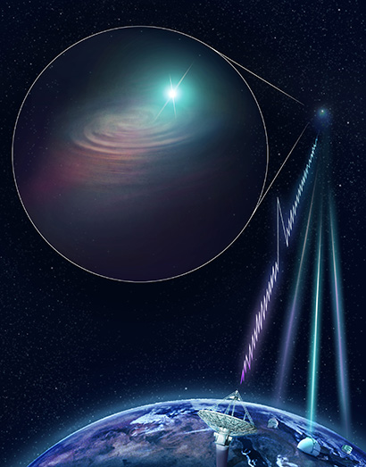
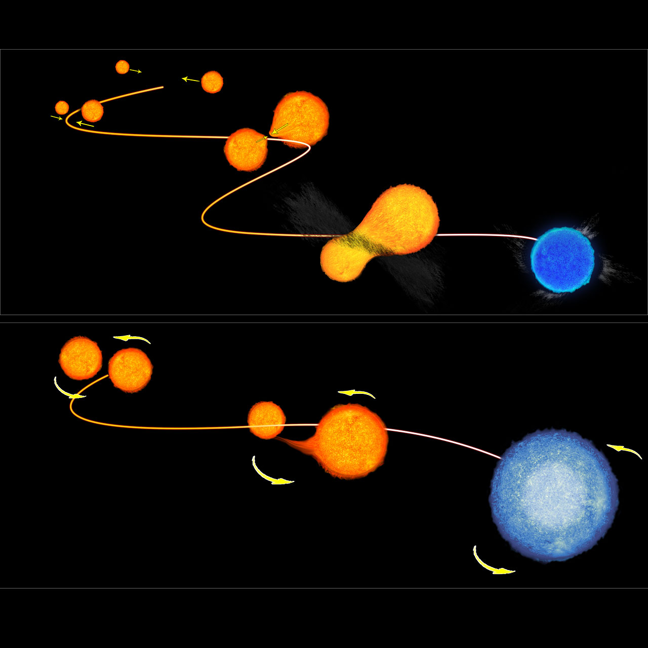
Artist’s illustration of a binary neutron star merger. [National Science Foundation/LIGO/Sonoma State University/A. Simonnet]
What We Saw and Why It’s Weird
On April 25, 2019, the LIGO detector in Livingston, Louisiana, spotted a gravitational-wave signal from a merger roughly 520 million light-years away. This single-detector observation — LIGO Hanford was offline at the time, and the Virgo detector in Europe didn’t spot it — was nonetheless strong enough to qualify as a definite detection of a merger.
Analysis of the GW190425 signal indicates that we saw the collision of a binary with a total mass of 3.3–3.7 times the mass of the Sun. While the estimated masses of the merging objects — between 1.1 and 2.5 solar masses — are consistent with the expected masses of neutron stars, that total mass measurement is much larger than any neutron star binary we’ve observed in our galaxy. We know of 17 galactic neutron star pairs with measured total masses, and these masses range from just 2.5 to 2.9 times that of the Sun. Why is GW190425 so heavy?
What It Suggests For Formation Channels

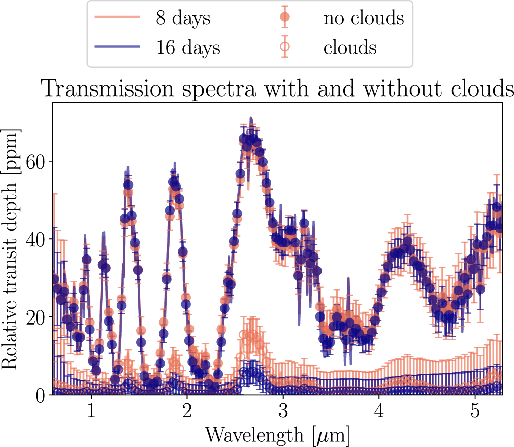
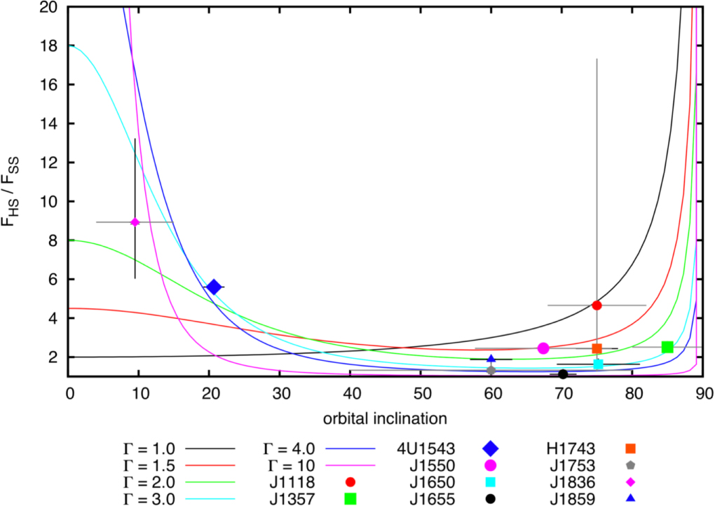
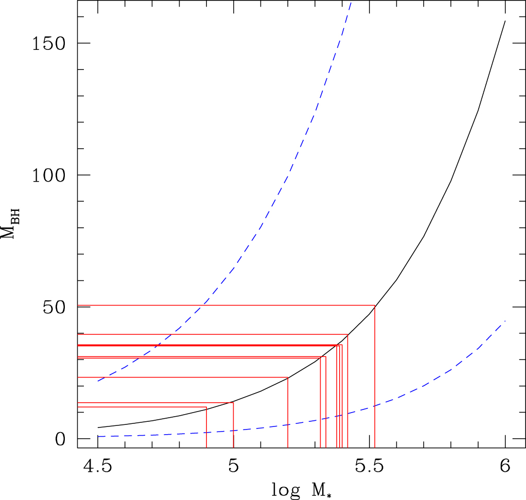
Blue and orange curves show the estimated total mass of GW190425 under different spin assumptions. In either case, the estimated mass is dramatically different from the total masses for the known galactic population of binary neutron stars, indicated with the grey histogram bars and the dashed line. [Abbott et al. 2020]
Theory suggests that massive, fast-merging neutron-star pairs like GW190425 could potentially result from especially low-metallicity stars evolving in close binary systems. Under the right conditions, the energetic kicks caused by supernova explosions might be suppressed, allowing the objects to stay together in the close binary even after their evolution into neutron stars.
If this is the case, GW190425 could represent a population of binary neutron stars that we haven’t observed before. These binaries have remained invisible due to their ultra-tight orbits with sub-hour periods; the rapid accelerations of these objects would obscure their signals in pulsar surveys. The shortest-period neutron star binary we’ve detected with pulsar surveys has a period of 1.88 hours, and it won’t merge for another 46 million years. GW190425 could represent a very different binary neutron star population that’s just as common as the galactic population we know.
What If It’s Not Neutron Stars?
Unfortunately, the single-detector observation of GW190425 means we couldn’t pin down the gravitational-wave source’s location well — so follow-up observations haven’t yet spotted an electromagnetic counterpart like the one we had for GW170817, the first binary neutron star merger LIGO observed.
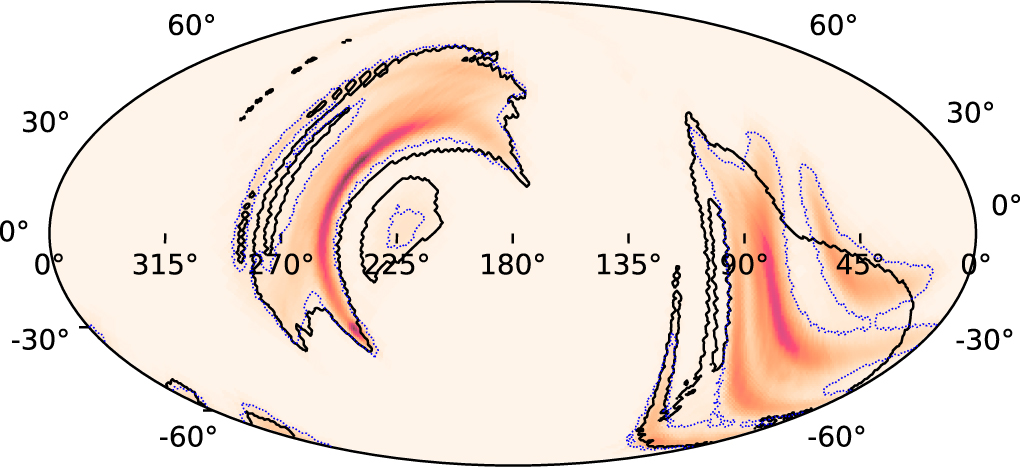
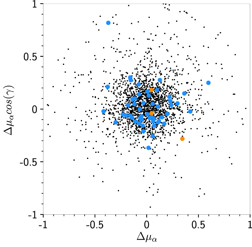
GW190425’s signal was localized to an unfortunately large area of ~16% of the sky, providing a challenge for electromagnetic and neutrino observatories hoping to discover counterparts. [Abbott et al. 2020]
There are clearly still a lot of open questions, but it’s early days yet! With the many recent upgrades to the LIGO and Virgo detectors, we can hope for more binary neutron star detections soon — and every new signal brings us a wealth of information in this rapidly developing field.
Citation
“GW190425: Observation of a Compact Binary Coalescence with Total Mass ~ 3.4 M⊙,” B. P. Abbott et al 2020 ApJL 892 L3. doi:10.3847/2041-8213/ab75f5


