Features RSS

A photograph of a bright white dot trailed by a fainter white stream.

A bold NASA experiment demonstrated that when an asteroid runs into something really hard, all of the ejected material reflects extra light back to Earth and makes the bruised asteroid appear slightly brighter for a short time. Recently, astronomers have built on that finding to estimate the chances of observing a similar flash out in the wilds of the main belt when two asteroids bump into each other by chance.

A DART of Inspiration

Back in September of 2022, NASA did its best to avenge the dinosaurs by slamming a small spacecraft into the moon of an asteroid. Aside from their vindictive motives, the agency had another, slightly more important reason for such an aggressive act. Astronomers and planetary defense experts wanted to watch how the asteroid would respond to a high-speed collision, and knowing exactly when one would occur allowed them to be ready with their telescopes. The Double Asteroid Redirection Test (DART) mission, as it was called, was a fabulous success, and the scientists involved got plenty of data along with the satisfaction of carrying out revenge 65 million years in the making.

A close-up view of the aftermath of the DART impact captured by a nearby spacecraft. [ASI/NASA/APL]

Moments after the spacecraft plowed into its target, the presumably surprised asteroid seemed to grow rapidly brighter. This temporary flash was caused in part by ejecta rapidly fleeing the crash site and reflecting additional sunlight back to Earth. As the material dispersed and the asteroid continued on its slightly altered course, it faded back to its original brightness.

Now, many months after the initial excitement, a team of astronomers led by Eran Ofek, Weizmann Institute of Science, have hit upon a realization: if asteroids flash during a collision, could we detect the small blips caused by an impact between two natural asteroids, instead of an asteroid and a human-made spacecraft?

Estimating Collision Rates

To answer their question, Ofek and collaborators needed to combine the answers to two smaller questions. First, would these natural collisions be bright enough to observe from Earth? Second, how often would these collisions actually take place? Both questions are non-trivial to solve, though following the success of DART, the first was slightly easier to tackle.

The distribution of brighness and distance to potential asteroid collisions. [Ofek et al. 2024]

By scaling the actual light curve collected after the DART mission came to its abrupt conclusion, the team could establish what the artificial impact would have looked like had the spacecraft and its target been teleported to the main belt of asteroids. The second question about the frequency of these collisions was more challenging to answer. Unfortunately, astronomers have nearly no idea how common asteroids the size of DART are in the solar system, since asteroids that small don’t reflect enough light to be observable from Earth. Luckily, the larger asteroids that they can observe seem to follow a power-law distribution in size, so by extrapolating that empirical relation to smaller objects, they can get a sense of how many unseen asteroids swarm in the dark.

Potential for Discoveries

Combining their insights, the researchers established that about 7,000 asteroid collisions could be detectable every year, plus or minus about an order of magnitude. That’s thrilling, but also puzzling: if multiple asteroids slam into each other and flash every night, why haven’t we seen them? The team offered two solutions: first, we actually have detected this phenomenon, and collisions make up at least a subset of the three or so “active asteroids” that are spotted each year. Second, these flashes are just too short to be caught by standard surveys, which would have to observe the same spot in the sky at least twice in one hour to resolve the brightening. Happily, that means with the right survey design, we could potentially recover many more of these collisions. Perhaps in the years to come astronomers will observe asteroid collisions even when they aren’t the cause of them.

Citation

“Asteroid Collisions: Expected Visibility and Rate,” Eran O. Ofek et al 2024 AJ 167 190. doi:10.3847/1538-3881/ad2c03

the cratered surface of the dwarf planet Ceres

Many of the craters on the dwarf planet Ceres are home to deposits of water ice. New research examines the ice-trapping properties these cold, shadowed craters and finds that the ice must be surprisingly young.

Dwarf Planet Discoveries

aerial view of a crater wall on Ceres

The Dawn spacecraft captured this image of a crater wall on Ceres from an altitude of about 26 miles (43 kilometers). [NASA/JPL-Caltech/UCLA/MPS/DLR/IDA]

Ceres, the only dwarf planet in the inner solar system, is a rocky world roughly a quarter of the diameter of the Moon. Ceres is of great interest to researchers because it’s likely one of the few surviving protoplanets in the solar system, the others having been ejected from the solar system, destroyed through collisions, or incorporated into planets.

From 2015 to 2018, NASA’s Dawn mission examined Ceres from orbit, reaching an altitude as low as 22 miles (35 kilometers) above the dwarf planet’s surface. Dawn peered into the craters at Ceres’s poles, many of which never see direct sunlight during Ceres’s 4.6-Earth-year orbit around the Sun, and discovered ice on some of the shadowed crater floors. Now, researchers have examined the locations and properties of these ice deposits to estimate how long they’ve been present.

map of permanently shadowed regions at Ceres's north pole

The slope of the terrain surrounding Ceres’s north pole (grayscale) with the locations of permanently shadowed regions colored by the maximum obliquity at which they remain in shadow. Click to enlarge. [Schorghofer et al. 2024]

Crater Considerations

Norbert Schorghofer (Planetary Science Institute) and collaborators used a detailed model of Ceres’s shape based on Dawn data to predict which of Ceres’s craters remain shadowed as its axial tilt, or obliquity, changes. Influenced by tidal forces from the Sun and Jupiter, Ceres’s obliquity varies from 2 degrees to 20 degrees over the course of 24,000 years. The team found that when Ceres reaches its maximum obliquity, there are no crater floors that remain shadowed throughout a Ceres year.

To understand what this means for the history of ice deposits on Ceres, Schorghofer’s team estimated how long it would take for ice on Ceres disappear through sublimation, transitioning directly from solid to gas. They found that when exposed to direct sunlight, ice deposits on Ceres sublimate rapidly, disappearing at a rate of more than a centimeter per year. If sublimation rates were small, that could mean that ice on Ceres could survive for billions of years. Instead, this result means that Ceres’s ice can’t survive long when exposed to sunlight and must be young.

Young Ice

area of shadowed regions as a function of latitude and obliquity

The area of shadowed regions as a function of latitude and obliquity. When Ceres’s obliquity reaches 20 degrees, there are no places that remain shadowed all year. [Adapted from Schorghofer et al. 2024]

Currently, ice deposits exist in regions that remain shadowed until Ceres’s axial tilt reaches 10 degrees. The last time Ceres’s tilt reached that value was just 6,000 years ago, which means that the ice can be no more than 6,000 years old. That’s remarkably young for a 4-billion-year-old protoplanet! Where is this ice coming from?

Ceres contains a lot of ice hidden under just a few centimeters of rocky surface material, so anything that disturbs the surface, such as landslides or impacts, could expose the ice. The authors find that the most likely source of Ceres’s surface ice is an impact that created a temporary atmosphere that condensed into ice in its craters.

Finally, the authors looked into the possibility of other types of ice, such as carbon dioxide ice, lining crater floors on Ceres. Despite being incredibly cold, Ceres’s craters are too warm to trap gases other than water vapor as ice.

Citation

“History of Ceres’s Cold Traps Based on Refined Shape Models,” Norbert Schorghofer et al 2024 Planet. Sci. J. 5 99. doi:10.3847/PSJ/ad3639

photograph of the supernova SN 2022jox and its host galaxy

If caught just a few days later, SN 2022jox would’ve looked like just another ordinary core-collapse supernova, but early observations set it apart, revealing the gas expelled in the star’s final years.

The Extraordinary Made (More) Ordinary

illustration of a red supergiant star surrounded by thick circumstellar material

An illustration of a red supergiant star surrounded by thick circumstellar material. [NAOJ]

It was once considered extraordinary to be able to observe a supernova just hours after the first light from the explosion reached Earth. With the advent of new surveys that scan the sky and hunt tirelessly for such flashes, it’s no longer exceptionally rare to catch supernovae early on — but it’s still extraordinarily useful.

These once-elusive early observations give a critical look at what the star was up to before its collapse. Observations suggest that in the final years of their lives, many massive stars lose mass through winds or eruptions. In the first few hours or days after a supernova explosion, the expanding ejecta collides with the material previously lost by the star, creating a burst of short-lived emission lines called a flash spectrum. Once the flash spectrum fades, this crucial information about the star’s immediate surroundings is lost.

spectra of SN 2022jox

Spectra of SN 2022jox taken 0.8–9.9 days after explosion. Click to enlarge. [Andrews et al. 2024]

Early Observations

In a recent research article, Jennifer Andrews (NSF’s NOIRLab and Gemini Observatory) and collaborators analyzed the flash spectrum and light curve of the supernova SN 2022jox. The event was caught soon after exploding by the Distance Less Than 40 Mpc Survey, which aims to find supernovae in nearby galaxies (within about 130 million light-years) within one day of the explosion reaching Earth.

At just 0.8, 1.3, and 1.5 days after the explosion, spectra of SN 2022jox showed narrow emission lines from hydrogen, helium, carbon, and nitrogen. Using radiative transfer modeling, Andrews’s team found that the gas surrounding the supernova was likely lost by its progenitor star at the rate of a thousandth to a hundredth of a solar mass per year — a high value for a quiescent red supergiant star, but typical for other supernovae with flash features in their spectra.

Critical First Days

Multi-band light curves of SN 2022jox

Multi-band light curves of SN 2022jox. The right panel shows a zoom-in of the first week of data. Click to enlarge. [Andrews et al. 2024]

Just a few days later, SN 2022jox’s narrow spectral lines flattened out, and the supernova’s evolution in the days that followed was typical for a core-collapse supernova: its peak brightness, the time it took to reach peak brightness, and the way its color changed over time were all normal. This shows the importance of catching supernovae as soon as possible after explosion — without catching the flash spectrum in those critical first days, SN 2022jox would have looked like any other normal core-collapse supernova.

Months after SN 2022jox was detected, the authors saw evidence for the expanding supernova interacting with circumstellar gas once again. Taken together, the very early and very late observations of this supernova suggest that it may be common for circumstellar material to be present around “ordinary” supernovae, and observations over a wide time frame are needed to detect these cases.

Citation

“SN 2022jox: An Extraordinarily Ordinary Type II SN with Flash Spectroscopy,” Jennifer E. Andrews et al 2024 ApJ 965 85. doi:10.3847/1538-4357/ad2a49

illustration of a gamma-ray burst in a star-forming region

One of the fundamental tenets of Einstein’s special theory of relativity is that the laws of physics are the same regardless of your vantage point. New research suggests a way to probe for cracks in this theory with a subtle measurement of gamma-ray photons.

Testing Special Relativity

Special relativity, which describes how mass, space, and time behave for objects moving close to the speed of light, has weathered every experimental challenge that researchers have thrown at it. A key edict of relativity is Lorentz invariance, or the idea that the laws of physics don’t vary from observer to observer. Other theories don’t hold Lorentz invariance so dear; some theories of quantum gravity, like string theory, allow for Lorentz invariance to be broken at very high energies.

If Lorentz invariance is violated — if the laws of physics do depend on your frame of reference — it opens the door to a host of bizarre effects. For one, the speed of light would not be constant, but would instead depend on the energy of the photon! In a recent research article, Justin Finke and Parshad Patel (US Naval Research Laboratory) explored another potential consequence of Lorentz invariance violation that could affect measurements of gamma-ray photons.

schematic of the model

Schematic of the model showing the positions of Earth, the Sun, and incoming gamma rays. [Finke & Patel 2024]

Making Particles from Photons

Very rarely, two photons can interact to produce a particle and its antiparticle — for example, an electron and a positron. If Lorentz invariance is violated, it could change the likelihood of these rare photon–photon interactions and impact observations of distant gamma-ray sources.

Finke and Patel explored a possible way to search for Lorentz invariance violations by examining the interaction between gamma-ray photons from extragalactic sources and photons from the Sun. Their mathematical model describes the rate at which gamma rays interact with solar photons as a function of the gamma ray’s energy, the angle between the gamma-ray source and the Sun, and the energies at which Lorentz invariance is violated.

Identifying an Invariance Violation

The team found that the number of gamma rays that interact with other photons to produce particle–antiparticle pairs, called the absorption optical depth, can increase or decrease as a result of Lorentz invariance violation. Whether the optical depth increases or decreases depends on the energies of the interacting photons — in this case, solar photons. For interactions with solar photons, this effect potentially becomes important for incoming gamma rays with energies above 10 teraelectronvolts.

plot of absorption optical depth with and without Lorentz invariance violation

An example of how the absorption optical depth, τνν, can either increase or decrease relative to its behavior in absence of Lorentz invariance violation, depending on the photon energy. This example shows gamma-ray absorption by the extragalactic background light. Click to enlarge. [Finke & Patel 2024]

Testing this prediction requires observing a gamma-ray source when it’s just peeking out from behind the Sun, then observing the same source when it’s far from the Sun. Comparing these two measurements, taken when the effect is at its largest and smallest, respectively, gives a measure of the absorption optical depth when the source is close to the Sun. Finally, comparing the absorption optical depth to what is predicted by the authors’ model yields a measure of the Lorentz invariance violation.

That’s how the measurement would work in theory — but could our present tools make it a reality? As of now, not in a reasonable time frame: given the sensitivity and observing limitations of current detectors, such as the High-Altitude Water Cherenkov Observatory, it could take more than 30 years to detect invariance violation, should it exist. If existing detectors could be tuned to distinguish between gamma rays and high-energy charged particles, it could shorten that time frame to as little as 1.3 years.

Citation

“Probing Lorentz Invariance Violation with Absorption of Astrophysical γ-Rays by Solar Photons,” Justin D. Finke and Parshad Patel 2024 ApJ 965 44. doi:10.3847/1538-4357/ad3212

photograph of a Centaur second-stage rocket

Upcoming surveys will find dozens of near-Earth objects each night, but some of those objects will be space junk rather than asteroids. How will we tell the difference?

Masquerading as Asteroids

When humankind sent its first rocket toward the Moon 65 years ago, it marked the beginning of a long era of lunar exploration. Now, the cast-off rocket parts from decades of lunar missions are cropping up in an unexpected place: searches for near-Earth asteroids.

Phase angle and light curve of an artificial object mistaken for an asteroid

Phase angle (top) and light curve (bottom) of an artificial object mistaken for an asteroid. [Battle et al. 2024]

Several artificial objects have already been mistakenly cataloged as asteroids, and that number is likely to grow. More than 100 lunar missions are planned for the next decade, creating opportunities for more space debris to masquerade as natural near-Earth objects. Future surveys, like Rubin Observatory’s Legacy Survey of Space and Time that will be underway in 2025, will discover dozens of near-Earth objects every night. To probe ways to differentiate between asteroids and space debris, researchers have turned their astronomical tools toward a near-Earth object that is likely a rocket body discarded in 1966.

One Person’s Space Junk Is Another’s Research Opportunity

In 2020, a planetary defense survey discovered a candidate near-Earth object named 2020 SO. Later, dynamical studies suggested that rather than being an asteroid, 2020 SO is instead a discarded Centaur-D rocket body from NASA’s Surveyor 2 mission to the Moon. 2020 SO’s orbit is unusual for a natural object, and while it’s large, roughly 10 meters by 3 meters, it’s lightweight enough that just the gentle pressure of the Sun’s radiation can push it off course.

reflectance spectra of 2020 SO and two classes of asteroids

Reflectance spectrum of 2020 SO (black) compared to those of two types of asteroids (green and blue). The spectra are normalized at 0.7 μm. [Battle et al. 2024]

Adam Battle (University of Arizona) and collaborators observed 2020 SO to search for photometric or spectral signatures that could differentiate between artificial objects and asteroids. Using visible-light observations from the Large Binocular Telescope, Battle’s team showed that 2020 SO is redder than is typical for most asteroids.

Conversely, it’s close in color to three known Centaur-D rocket bodies in Earth orbit, although the colors don’t match perfectly. This suggests that if 2020 SO is also a Centaur-D rocket body, its surface has changed after decades of space aging from radiation and particle impacts.

Spectroscopy Has the Last Word

While it’s possible for artificial objects to be similar in color and reflectance to asteroids, spectroscopy lays their differences bare by revealing what they’re made of. A Centaur-D rocket body is largely covered in stainless steel and a polymer called polyvinyl fluoride, and its spectrum likely contains features from both materials. Using data from the Infrared Telescope Facility, Battle and coauthors compared the spectrum of 2020 SO to the spectrum of a known Centaur-D rocket as well as laboratory spectra of stainless steel and polyvinyl fluoride.

Infrared spectra of 2020 SO and a Centaur-D rocket body

Infrared spectra of 2020 SO (black) and a Centaur-D rocket body (green). [Battle et al. 2024]

The spectrum of 2020 SO is similar in shape to the spectrum of stainless steel, and 2020 SO sports a distinct absorption feature at 2.3 microns (1 micron = 10-6 meter), just like the spectrum of polyvinyl fluoride. Taken together, 2020 SO’s area-to-mass ratio, color, and spectrum all point to the object being a rocket body rather than an asteroid.

This study shows that photometry and infrared spectroscopy can reveal the colors and spectral features necessary to identify near-Earth objects. To take the identification of artificial objects a step further, future work may require a database of artificial-object spectra and laboratory studies of common spacecraft materials.

Citation

“Challenges in Identifying Artificial Objects in the Near-Earth Object Population: Spectral Characterization of 2020 SO,” Adam Battle et al 2024 Planet. Sci. J. 5 96. doi:10.3847/PSJ/ad3078

How do cosmic rays spread through the galaxy? Historically, that’s been a hard question to answer from within the Sun’s protective bubble that shields us from some fraction of these high-energy particles. However, now that Voyager 1 has completed its hard-fought journey into interstellar space, astronomers can study cosmic rays beyond the reach of the Sun to build a fuller picture of the lives of these lightning-fast bits of matter.

Tiny Bullets

A schematic of Voyager 1. The cosmic ray experiments are in the upper right. [NASA’s Goddard Space Flight Center]

Cosmic rays, or tiny chunks of atomic nuclei that whiz around at nearly the speed of light, permeate the entire Milky Way and the spaces between the galaxies. For nearly a century, astronomers have observed them flying through our own backyard, first via balloon experiments that caught them colliding with particles in Earth’s upper atmosphere, then later via satellites perched in orbit. Throughout the entire span of these observations, we’ve known that the cosmic rays we’ve recorded might not be representative of the broader population, since we only see those that managed to barrel into the inner solar system without being dissuaded by the protective influence of the Sun. This has made it challenging to model how cosmic rays flow through space in general, and consequently harder to constrain where they all come from.

For about a decade, however, astronomers have been able to call upon a hardy scout that has flown beyond the reaches of our Sun and into the region where cosmic rays roam free. Voyager 1, launched an astounding 46 years ago and still limping along despite recent communication challenges, was the first human-made object to reach interstellar space back in 2012. Even as the spacecraft shut down other instruments to ration its limited power source, it kept its cosmic ray experiments powered up and collecting data. Now, by combining measurements from Voyager 1 with data collected by instruments on the International Space Station, astronomers can revisit their models of how cosmic rays move through the galaxy and within our solar system.

The Alpha Magnetic Spectrometer after its installation aboard the International Space Station. [NASA]

Many Models Mostly Working

Ethan Silver, University of California Berkeley, and Elena Orlando, University of Trieste, recently attempted this comparison. Using about a decade’s worth of data from Voyager 1 and from the Alpha Magnetic Spectrometer aboard the International Space Station, they were able to fit six different types of models of how cosmic rays move through the galaxy, each with many parameters that needed to be carefully tuned. Some of these models assumed that one can capture the behavior of cosmic rays using only a diffusion framework, while others were much more complex and allowed for numerous discontinuities in the input spectra of energies for each type of particle.

Silver and Orlando found that in general, all of the models they tested could explain the observed data with reasonable success. Though unsurprisingly the more complex models with more free parameters agreed with the measurements the best, the lighter-weight models held their own and couldn’t be confidently ruled out. Interestingly, all of the models tested failed on the same subset of observations: none of the schemes they tested, including the most complex diffusion-convection-reacceleration models, accurately predicted the flux of antiprotons with energies around ∼10 giga-electron volts. This missed prediction suggests that even with the help of probes far beyond our confines here on Earth, there is still much we don’t know about the production and transportation of cosmic rays. However, the general success of the models indicates that we’re on the right track, a validation enabled in large part by a distant and aging but well-loved spacecraft.

Citation

“Testing Cosmic-Ray Propagation Scenarios with AMS-02 and Voyager Data,” Ethan Silver and Elena Orlando 2024 ApJ 963 111. doi:10.3847/1538-4357/ad1ce8

photograph of the rings of Saturn and five of Saturn's moons

The giant planets in our solar system — Jupiter, Saturn, Uranus, and Neptune — collectively host nearly 300 moons. What can craters tell us about how old these moons are and how they formed?

How Are Moons Made?

submillimeter-wavelength image of the PDS 70 planetary system, which contains a circumplanetary disk

A submillimeter image of the PDS 70 planetary system. Between the outer ring of gas and the central star sits the Jupiter-like exoplanet PDS 70c, which is surrounded by a possible moon-forming circumplanetary disk. [ALMA (ESO/NAOJ/NRAO)/Benisty et al.; CC BY 4.0]

Theories of how the solar system’s many satellite worlds came to be are nearly as varied as the satellites themselves. The leading theory is that disks of gas, dust, and pebbles surrounding newborn planets provided the material for moons to form, much like how planets form out of gas and dust surrounding a newborn star. Other theories suggest that massive ring systems around giant planets are the sites of moon formation, or that some satellites coalesce from the debris of previous satellite collisions.

Crater counting provides a way to estimate the ages of satellite surfaces — placing limits on the ages of the objects themselves — and helps test these theories of satellite formation. To understand how the craters on a moon’s surface relate to the age of the surface, researchers had to imagine conditions in the solar system nearly 4.5 billion years ago, when things were far more chaotic than they are today.

plot of cumulative number of impactors versus impactor size

Modeled cumulative number and size of impactors striking giant planet satellites since the beginning of the bombardment period. Satellites with similar collision probabilities are grouped together for clarity. Click to enlarge. [Bottke et al. 2024]

Shuffling the Solar System

A few tens of millions of years after the gaseous nebula that enveloped the young Sun and its budding planets dissipated, Neptune shook up the solar system. As Neptune migrated outward from the Sun, it crossed into a primordial disk of planetesimals, kicking 99.9% of these icy bodies into the solar system. (The remaining 0.1% of planetesimals remained behind and formed what is today known as the Kuiper Belt.) Thus began a long period of bombardment that is recorded on the surfaces of the many moons of the outer solar system.

Recently, William Bottke (Southwest Research Institute) and collaborators assigned ages to the surfaces of 26 satellites of Jupiter, Saturn, Uranus, and Neptune by modeling crater formation during this bombardment period.

To measure surface ages from the craters observed on these satellites today, the team modeled the sizes and numbers of craters forming due to bombardment on each satellite as a function of time. This model accounts for the relationship between the size of the impacting body and the size of the crater, changes in the sizes of the impacting bodies over time due to collisions between impactors, and other factors.

Missing Early History

modeled and observed crater size and frequency values

Modeled (black lines) and observed (colored circles) crater size and frequency values for several small moons. The derived surface ages are listed in each panel. Bombardment begins at T = 20 million years after the gas disk disperses. Click to enlarge. [Bottke et al. 2024]

All of the satellites in the study were missing evidence of the large impacts that should have occurred early on in the bombardment period. This suggests that the satellites were resurfaced through surface melting, shattering, or total disruption of the object, hiding these large early craters. The oldest surfaces, belonging to Iapetus, Hyperion, Phoebe, and Oberon, go back to just a few million years after the bombardment began, while the youngest surfaces, belonging to the largest moons, could be billions of years younger.

With early history erased by large impacts, it’s not possible to definitively state how these worlds formed — though Bottke’s team notes that for midsize and large moons, their model results are consistent with what’s expected for satellites forming in a disk around their host planets. Significant roadblocks exist for other theories. If future spacecraft can make sensitive gravity measurements of these worlds, revealing bombardment-induced changes to their crusts and interiors, it could reveal this hidden era of solar system history.

Citation

“The Bombardment History of the Giant Planet Satellites,” William F. Bottke et al 2024 Planet. Sci. J. 5 88. doi:10.3847/PSJ/ad29f4

phases of a total solar eclipse

Today’s the day! The Moon’s shadow will sweep across Mexico, the United States, and eastern Canada, plunging millions of eclipse viewers into a few minutes of mid-afternoon twilight. I’ll be enjoying a partial eclipse in partly cloudy Colorado, having bailed on my original plans for totality in Texas due to thunderstorms. See you all in Spain in August 2026, perhaps?

Whether your plans have been sidelined by weather or you’re enjoying the eclipse under sunny skies, take a moment to delve into three solar physics research articles with us today to learn how researchers are studying our home star.

Launching the Solar Wind with Tiny Jets

The solar wind is a hot, tenuous plasma that constantly streams out from the Sun, whipping past Earth at about 400 kilometers per second. How the solar wind is launched from the Sun’s atmosphere is a hot topic, with recent research suggesting that thousands of small jets powered by the release of pent-up magnetic energy could provide the boost the solar wind needs to get going.

plot of number of events versus size of events for erupting filament-like features on the Sun

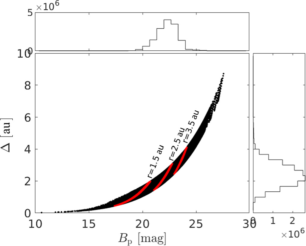
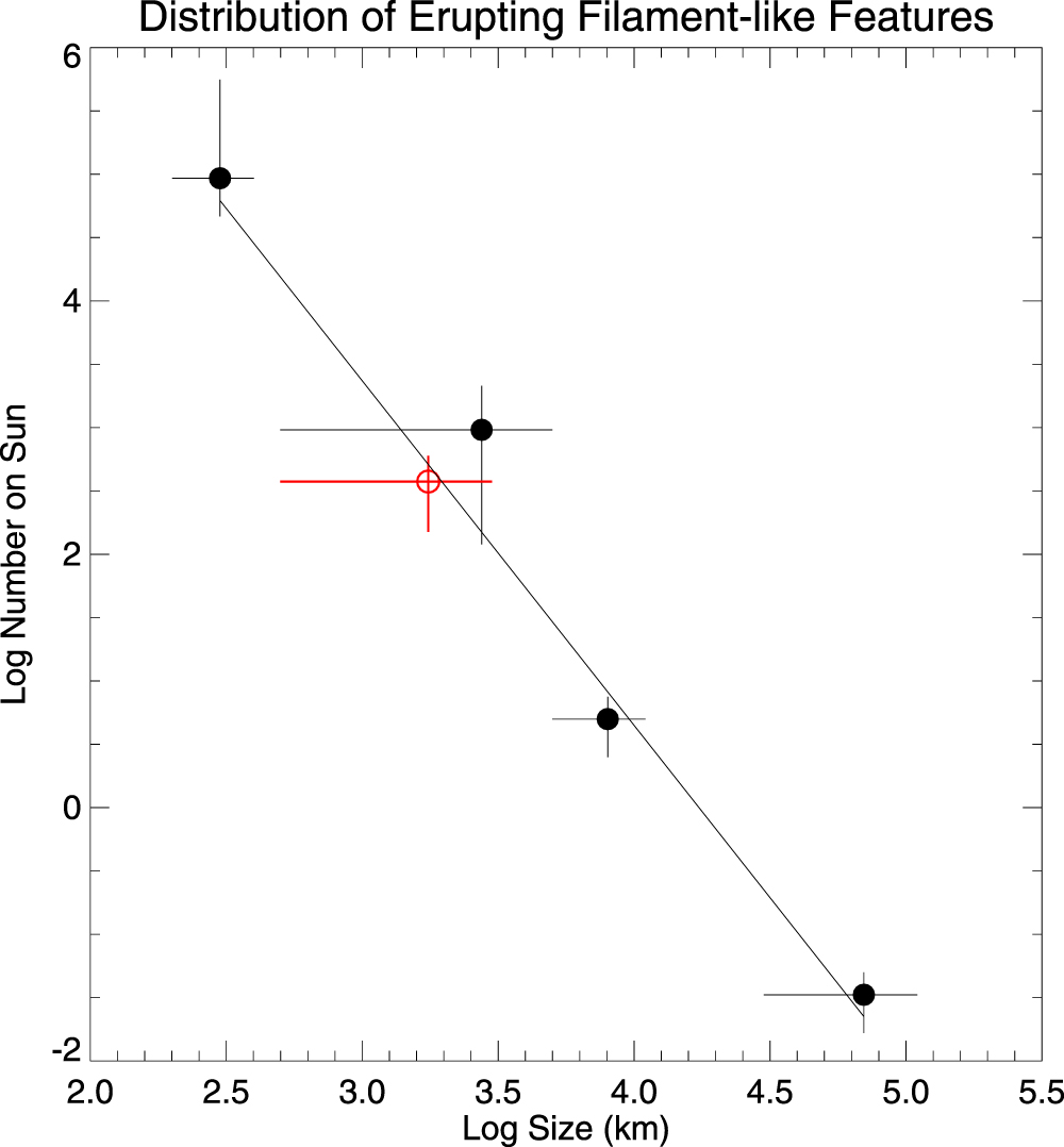
Number and size distribution of erupting filaments on the Sun. From left to right, the black circles represent microfilament eruptions, jetlets, minifilament eruptions, and solar flares and coronal mass ejections. [Sterling et al. 2024]

Recently, 
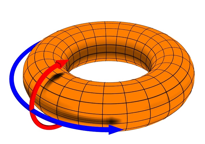
Alphonse Sterling (NASA’s Marshall Space Flight Center) and collaborators examined the physics behind this hypothesis. Coronal jets and their smaller counterparts, jetlets, seem to be associated with the eruption of loops of coronal plasma called filaments. Sterling’s team cataloged a wide range of solar phenomena, from tiny minifilaments that span just a few thousand kilometers (“tiny” is relative!) to huge coronal mass ejections that shrug off the Sun’s gravity and explode into space. The team found that the sizes and occurrence rates of these coronal structures fall along a power law, suggesting that they may all be triggered by the same mechanism: the eruption of a twisted tube of magnetic fields called a magnetic flux rope.

Looking more closely at the connection between jets and the solar wind, Sterling’s team proposed that when a flux rope erupts, the material ensnared within the rope is launched outward, and the intrinsic twist of the magnetic field in a flux rope could be transferred to field lines that extend out into the solar system. The movement of this magnetic field twist could produce magnetic zigzags called switchbacks, which have been observed in detail by the Parker Solar Probe and Solar Orbiter, connecting the beginnings of the solar wind to phenomena seen farther downwind.

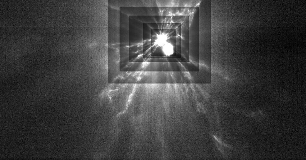
A Coronal Mass Ejection Seen from Mercury, Earth, and Other Locations in Space

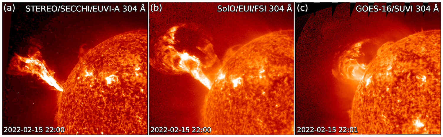
With spacecraft orbiting Earth, zooming around other planets, and even skimming the Sun’s atmosphere, we can study the Sun from more angles than ever before. In February 2022, three spacecraft made ultraviolet observations of a loop of solar plasma suspended within the Sun’s magnetic field. The loop of plasma, called a prominence, eventually erupted as a coronal mass ejection. The BepiColombo spacecraft and the Parker Solar Probe weathered the coronal mass ejection from their positions near Mercury’s orbit, just 0.35 au from the Sun.

three extreme-ultraviolet images of the Sun, showing different perspectives on an erupting filament

Three extreme-ultraviolet viewpoints of the same event on 15 February 2022. From left to right: the STEREO spacecraft, at Earth’s orbital distance; Solar Orbiter, around 0.75 au; and the GOES spacecraft, in orbit around Earth. [Palmerio et al. 2024]

As the fleet of spacecraft exploring our solar system grows, it has become more common for coronal mass ejections to interact with multiple spacecraft (although it’s still quite rare!). This event gave researchers an exceptional opportunity to study coronal mass ejections, as BepiColombo and the Parker Solar Probe were separated by only a few million kilometers and were only a small angular distance apart.

This allowed Erika Palmerio (Predictive Science Inc.) and collaborators to study how the structure of a coronal mass ejection varies on these scales. Despite the small separation of the spacecraft, many of the properties they measured were considerably different. For example, they measured different directions of the shock as it passed over them, and the time it took for the coronal mass ejection to pass over them was measured to be different by more than 9 hours. This reveals that coronal mass ejections have considerable variations over the scales examined in this study, and more work is needed to understand how and why these variations exist.

A Potential Solution to a Persistent Problem

Magnetic field lines that emerge from the Sun’s surface and loop back to re-enter the surface are called closed field lines, while those that extend out into the solar system are called open field lines. For decades, researchers modeling the solar corona have encountered a persistent issue: models predict far less open magnetic flux than spacecraft measure. The discrepancy can be a factor of two or more, and the mismatch tends to be greatest when modeling the Sun at its most active.

comparison of open magnetic flux observations and derived measurements

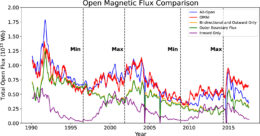
Comparison of the observed open magnetic flux (red line) with the results of various methods of tallying the flux. The blue line shows the results of the method explored in this study. Click to enlarge. [Arge et al. 2024]

A research team led by C. Nick Arge (NASA’s Goddard Space Flight Center) has proposed that the solution to this problem lies at the boundaries between regions of open and closed field lines. Arge’s team showed that the traditional method of summing up regions of open magnetic flux at the outer boundary of the model — around 2.5 solar radii — undercounts the amount of open flux, while a method that relies on tracing the magnetic field from the outer boundary down to the solar surface and from the solar surface to the outer boundary nearly matches the observed values.

The mismatch between the two methods is greatest when the grid cells of the model fall upon an active region — an area of especially strong and complicated magnetic fields — that lies on the edge of a coronal hole, where a concentration of open magnetic field lines carries solar plasma into space. This fact hints at why previous methods were least successful in matching the observed open flux when the Sun was active; high solar activity means more active regions, and more opportunities to miss open flux.

While the new method hasn’t yet been perfected, tending to overestimate the open magnetic flux in some cases, the authors hope that it will finally bring the open flux mystery to a close.

Citation

“How Small-Scale Jetlike Solar Events from Miniature Flux Rope Eruptions Might Produce the Solar Wind,” Alphonse C. Sterling et al 2024 ApJ 963 4. doi:10.3847/1538-4357/ad1d5f

“On the Mesoscale Structure of Coronal Mass Ejections at Mercury’s Orbit: BepiColombo and Parker Solar Probe Observations,” Erika Palmerio et al 2024 ApJ 963 108. doi:10.3847/1538-4357/ad1ab4

“Proposed Resolution to the Solar Open Magnetic Flux Problem,” C. Nick Arge et al 2024 ApJ 964 115. doi:10.3847/1538-4357/ad20e2

Illustration of a dusty accretion disk surrounding the supermassive black hole at the center of a galaxy

Do models of turbulent, magnetized gas in accretion disks around black holes “remember” the conditions they started with, or is that information washed away as the model evolves?

Magnetic Fields and Accretion Disks

If you’re an astronomer, you may already know this joke: an astronomer is speaking with a therapist, discussing a recent bout of sleeplessness. The therapist asks, “What do you think it is that’s keeping you up at night?” Staring wide-eyed at the ceiling, the astronomer whispers, “Magnetic fields…”

Today’s article presents one example of why astronomers might lose sleep over magnetic fields. Magnetic fields are a key component of accretion disks, which feed material to growing stars, black holes, and other objects. Researchers have had great success in modeling magnetized accretion disks, but the huge computational cost of increasingly complex models has prompted the use of time-saving shortcuts with the potential for unintended side effects.

Testing a Model’s Memory

One way to speed up simulations is to start out with the model’s magnetic fields close to the desired end state. Recently, Payton Rodman (University of Cambridge) and Christopher Reynolds (University of Cambridge and University of Maryland) tackled the question of whether it matters what kind of magnetic fields a model starts with when simulating accretion disks around supermassive black holes.

illustration of poloidal and toroidal directions

Illustration of the poloidal (red arrow) and toroidal (blue arrow) directions. [Wikipedia user DaveBurke; CC BY 2.5]

Our best observations of supermassive black holes suggest that the magnetic fields close to the black hole are strong and poloidal, meaning that the fields are vertical close to the black hole and arc up over the disk. These strong poloidal fields are thought to be responsible for launching powerful black hole jets.

To save time, many models start out with a strong poloidal magnetic field. However, real accretion disks might instead start out with weak toroidal magnetic fields, which circle the black hole horizontally. If all magnetic fields, regardless of initial strength of configuration, “forget” their initial state and eventually evolve into the strong poloidal fields that researchers observe, that means that modelers can choose any reasonable starting parameters. If the magnetic fields retain a memory of their initial state, modelers will need to carefully examine their starting conditions and how the fields evolve.

A Clear Imprint

Rodman and Reynolds compared the evolution of weak and strong toroidal magnetic field models to test the “memory” of their accretion disk model. They found that the weak and strong magnetic field simulations diverged quickly and didn’t reach the same end point — the final outcome retained an imprint of the initial field strength.

plot of magnetic field streamlines from the simulation results

Magnetic field streamlines for simulations with a weak initial magnetic field (left) and a strong initial magnetic field (right). Click to enlarge. [Rodman & Reynolds 2024]

Ultimately, the weak and strong toroidal magnetic fields both produced poloidal fields, but how strong the fields were and how widely they were distributed depended on the initial field strength. Critically, neither simulation generated poloidal fields strong and widespread enough to reach the magnetically arrested disk regime, which is thought to govern how supermassive black holes at the centers of galaxies accrete matter and produce jets.

The results of this study make it clear that initial magnetic field conditions must be chosen carefully, as accretion models appear to have long memories. Future work should delve into this issue further, hopefully helping astronomers everywhere to rest easier.

Citation

“Evolution of the Magnetic Field in High- and Low-β Disks with Initially Toroidal Fields,” Payton E. Rodman and Christopher S. Reynolds 2024 ApJ 960 97. doi:10.3847/1538-4357/ad0384

Illustration of a blue supergiant star

New research shows that the properties of some blue supergiant stars can be explained by the merger of a massive star with a smaller companion. This suggests that many of the brightest and hottest stars in our galaxy are not born, but made.

One Star or Two?

JWST image of SN 1987A

JWST image of SN 1987A. Some research suggests that the intricate ejecta pattern could not be possible without the supernova progenitor star undergoing a merger. [NASA, ESA, CSA, Mikako Matsuura (Cardiff University), Richard Arendt (NASA-GSFC, UMBC), Claes Fransson (Stockholm University), Josefin Larsson (KTH)]

The blue supergiant stage is a brief phase in the lives of hot, massive stars. Though the phase is short-lived, there seem to be a lot of blue supergiants, and despite the fact that massive stars tend to live in pairs or trios, there seem to be a lot of supergiants without a stellar partner. These curious findings could be explained by a scenario in which some blue supergiants form when a massive star swallows its companion.

Researchers have applied this line of thinking to several famous massive stars like Eta Carinae and the progenitor of the supernova SN 1987A, showing that the merger model explains these stars’ unusual properties. Now, a research team led by Athira Menon (Institute of Astrophysics of the Canary Islands and University of La Laguna) has taken the investigation a step further, using this model to explain the varied properties of a population of blue supergiant stars in a neighboring galaxy.

evolutionary track of a stellar merger product

Evolutionary track for the merger product of a 31.6-solar-mass star and a 3.2-solar-mass star. [Menon et al. 2024]

A Star Is Made

Menon’s team used the Modules for Experiments in Stellar Astrophysics (MESA) to model the evolution of post-merger stars and to compare the properties of blue supergiants coming from single stars to those coming from stellar mergers.

In the stellar merger scenario, blue supergiants result from the collision of a massive post-main-sequence star and its main-sequence binary companion. As the massive star expands, it donates some of its mass to its companion, which eventually becomes entangled in the extensive outer atmosphere of the larger star. Doomed by friction and tidal forces, the smaller star “dissolves” within the larger star, setting the resulting star on a new evolutionary path.

Clues from Chemical Abundances

The team found that blue supergiants formed through mergers have different surface abundances of elements like carbon and oxygen compared to supergiants arising from single stars. To compare these results to the properties of actual blue supergiants, the team amassed a sample of 59 blue supergiant stars in the Large Magellanic Cloud and divided them into three groups based on the ratios of their carbon, nitrogen, and oxygen abundances.

chemical abundances of modeled and observed blue supergiants

Chemical abundance ratios for modeled stars (star icons) and observed blue supergiants (BSGs; triangles). Click to enlarge. [Menon et al. 2024]

The first group, which had relatively little nitrogen compared to carbon and oxygen, matched the outcomes of the single-star models — these stars are likely “true” blue supergiants that evolved from single stars. The second group, with moderate N/C and N/O ratios, could be explained by either single stars or stellar mergers. The final group, which made up about 40% of the sample, had larger abundance ratios that the single-star model couldn’t reproduce.

Taking into account other factors, such as systematic offsets, Menon’s team concluded that more than half of the 59 stars in their sample came from stellar mergers. This suggests that many blue supergiant stars owe their status to a stellar merger, and the merger model is a valuable tool to understand blue supergiant populations throughout the universe.

Citation

“Evidence for Evolved Stellar Binary Mergers in Observed B-type Blue Supergiants,” Athira Menon et al 2024 ApJL 963 L42. doi:10.3847/2041-8213/ad2074

1 14 15 16 17 18 111