Features RSS

supernova

A kilometer below Japanese ground lies a massive cylindrical tank, its steel walls lined with more than 10,000 photomultiplier tubes that await the arrival of neutrinos. Could recent upgrades to the Super-Kamiokande neutrino detector improve our ability to spot and assess supernova explosions in real time?

JWST image of SN 1987A

JWST image of SN 1987A. The optical signal of this explosion was preceded by the arrival of a burst of neutrinos, a handful of which were observed by detectors on Earth. [NASA, ESA, CSA, Mikako Matsuura (Cardiff University), Richard Arendt (NASA-GSFC, UMBC), Claes Fransson (Stockholm University), Josefin Larsson (KTH)]

Memo from a Dying Star

In 1987, 25 tiny messengers arrived at Earth following a tremendous explosion 168,000 light-years away. This signal marked the first time that these near-massless messengers — neutrinos — had ever been directly observed from a Type II supernova, the core collapse of a massive star.

The benefit of observing these particles is clear: because neutrinos so rarely interact with matter, they arrive at Earth carrying untouched information about the death of the star that produced them. And because neutrinos escape the collapsing star more readily than photons do, they arrive before the visible light from the supernova. This means that if scientists can detect and localize a supernova neutrino burst, they can notify observatories about the imminent optical signal from the supernova. Combining the neutrino and electromagnetic observations could then provide valuable insight into long-standing questions, like the mechanism of the star’s explosion.

The catch? We only expect a handful of nearby (i.e., in our galaxy) supernova explosions every century — and what’s more, observing neutrinos is no easy feat! In the nearly four decades since those 25 messengers heralded the supernova SN 1987A, we haven’t detected any other neutrinos linked to supernovae. But that doesn’t mean we haven’t been preparing.

A Salty Upgrade for Super-K

Super-Kamiokande scale model

A scale model showing the (empty) tank of the underground Super-K neutrino detector. A recent upgrade saw a gadolinium salt added to the water that fills the tank. [Adapted from Wikipedia user Motokoka; CC BY-SA 4.0]

The Super-Kamiokande (Super-K) neutrino detector has recently undergone an upgrade: scientists have dissolved a gadolinium salt in the 55,000 tons of ultrapure water that fills its underground tank. The addition of this rare-earth metal improves the detector’s ability to differentiate between neutrinos and antineutrinos, thereby enabling scientists to more accurately localize the supernova that produced an incoming burst of neutrinos.

In a recent article led by Yuri Kashiwagi (Kamioka Observatory, Institute for Cosmic Ray Research, University of Tokyo), Super-K scientists have analyzed how this upgraded observatory — and a corresponding real-time alert system developed to notify optical astronomers of the explosion and tell them where to point their telescopes — will respond to a hypothetical supernova within our galaxy.

Passing the Message On

Using multiple different supernova models, Kashiwagi and collaborators simulated the neutrino burst that would be produced by a supernova exploding roughly 33,000 light-years away. Through further simulations, the team then explored how successfully Super-K would detect neutrinos from the burst, how well the supernova’s location could be identified from Super-K’s detections, and how quickly this information could be broadcast to astronomical observatories via the alerting system.

supernova localization

The blue contours on this sky map show an example of the reconstructed supernova position that Super-K neutrino observations should provide for a supernova that occurs 33,000 light-years away. In this example, the supernova’s location can be identified to within 3°. [Adapted from Kashiwagi et al. 2024]

The authors found that the simulated supernova’s location could be rapidly identified to within 3–7° on the sky, and that information could be sent to optical observatories within minutes. In many cases, this response would be sufficient for wide-field telescopes like the upcoming Vera Rubin Observatory to catch the rise of the optical signal from a supernova — and the neutrino data captured by Super-K could even help distinguish between different supernova models.

While there’s still more to learn, it seems likely that Super-K is well prepared for future nearby supernova detections. Now all that’s left is to wait for the next explosion!

Citation

“Performance of SK-Gd’s Upgraded Real-time Supernova Monitoring System,” Y. Kashiwagi et al 2024 ApJ 970 93. doi:10.3847/1538-4357/ad4d8e

JWST photograph of the Cartwheel Galaxy

Today’s Monthly Roundup is a bit of an astrophysical mishmash, highlighting some of the structures that exist in our universe. From galaxies to planets, we’ll explore where these structures come from and the tools researchers use to study them.

A Ring Galaxy

When gamma-ray telescopes like Fermi survey the sky, they see discrete sources of gamma rays as well as a diffuse background glow. Discerning exactly where these gamma rays come from is no easy task, and roughly 30% of known gamma-ray sources haven’t been identified. Many of these unassociated sources are likely active galactic nuclei (AGN) — accreting supermassive black holes that can launch powerful jets — but some may have more unusual origins.

annotated ultraviolet image of Kathryn's Wheel

An ultraviolet image (background color) of the Kathryn’s Wheel system with contours showing the Hα emission. Annotations have been added to show the various components of this system. Click to enlarge. [Adapted from Paliya & Saikia 2024]

In a recent article, Vaidehi Paliya and D. J. Saikia (Inter-University Centre for Astronomy and Astrophysics) matched the gamma-ray source 4FGL J1647.5−5724 to a galaxy called Kathryn’s Wheel. Kathryn’s Wheel is a ring galaxy, consisting of a central gas-poor galaxy surrounded by a ring of star formation. This curious system likely formed when a nearby dwarf galaxy, LEDA 3080069, shot through it like a bullet, kicking gas out of the system and triggering a shock wave that kick-started star formation in a ring around it.

Multiwavelength images of Kathryn’s Wheel show bright Hα and ultraviolet emission, both of which signal the presence of hot, massive young stars. Intense star-forming regions are known to emit gamma rays, in part because of the frequent core-collapse supernovae that shock interstellar gas and accelerate cosmic rays. A closer look at the galaxy revealed that its gamma-ray emission is stronger than expected, suggesting either a population of rapidly spinning stellar remnants called pulsars or — as a more mundane explanation — interference from a foreground Milky Way star.

In addition to triggering star formation, galaxy collisions can also activate AGN. While the current data show no signs of gamma-ray variability or relativistic jets — both of which would indicate an AGN — more observations are needed to look into the possibility further.

High-Energy Bubbles

In 2010, scientists discovered that the Milky Way has been blowing bubbles. Observations with the Fermi Gamma-ray Space Telescope revealed bubbles of gamma-ray emission extending 50 degrees above and below the plane of our galaxy. Ten years later, the eROSITA instrument on the Spectrum-Roentgen-Gamma spacecraft spotted a similar but even more extensive structure in X-rays. The origin of these structures, called the Fermi and eROSITA bubbles, is not yet known. Many researchers have suggested that a past period of AGN activity, in which the Milky Way’s central supermassive black hole accreted matter and shot out powerful jets, could be responsible.

Recently, Po-Hsun Tseng (National Taiwan University) and collaborators approached the AGN activity hypothesis from a new angle. Previous work has tested this theory under the assumption that the AGN jets emerged vertically from the plane of the galaxy, matching the orientation of the bubbles. However, this doesn’t have to be the case — the direction of an AGN’s jets is related to the spin of the black hole, which doesn’t have to be parallel to the galactic disk.

simulated gamma-ray bubbles

Simulated gamma-ray bubbles from jets emerging perpendicular to the disk (top), at a 45-degree angle to the disk (middle), and parallel to the disk (bottom). [Adapted from Tseng et al. 2024]

Using special relativistic fluid dynamics simulations, Tseng’s team examined whether angled AGN jets could produce vertical bubbles. The simulated jets emerged from the plane of the Milky Way at a 45-degree angle, remaining “on” for 120,000 years before shutting off. A key component of the team’s model is the inclusion of a thin, dense, clumpy layer of interstellar gas lying parallel to the galactic disk. When the jet collides with this layer, interactions between cosmic rays in the jet and gas within the layer produce gamma rays.

Ultimately, the team found that under certain conditions, the jets transfer their kinetic energy to the dense layer of gas without plowing through it, and the once-narrow jets instead emerge vertically from the disk as bubbles. While more modeling is needed to understand the origin of the Fermi and eROSITA bubbles, this work shows that the assumption of vertical jets need not apply.


A Chain of Planets

When planets form in the dusty recesses of a protoplanetary disk, their motions within the disk are thought to align the planets in a resonant chain: a setup in which the orbital periods of the planets are integer multiples of one another. For example, a three-planet system with 8-, 16-, and 32-day orbits would be in a resonant chain. If planets do link up in resonant chains when they first form, something — gravitational nudges from passing stars, for example — must break those chains, as only 1% of known planetary systems are in this configuration. It’s critical to identify the small percentage of systems with intact resonant chains since they show the initial state of a planetary system before it’s disrupted.

plot of the cumulative fraction of unstable systems over time

Cumulative fraction of simulated six-planet systems becoming unstable as a function of time. Nearly all non-resonant systems are unstable by 25 million years, while only a small fraction of six-planet resonant chains go unstable in that same stretch of time. Click to enlarge. [Lammers & Winn 2024]

Caleb Lammers and Joshua Winn (Princeton University) investigated a potential resonant chain in the HD 110067 system. If confirmed, HD 110067 would be just the third known resonant chain containing six or more planets. HD 110067 has six known transiting planets with orbital periods between 9.1 and 55 days. The planets’ orbital periods are very nearly in ratios of 3:2 and 4:3 — highly suggestive of a resonant configuration.

Lammers and Winn performed N-body simulations to assess the likelihood that the system is arranged in a resonant chain. They found that in order for HD 110067’s six planets to be dynamically stable, the planets almost certainly must be in a chain. Simulated non-resonant systems become unstable within 25 million years — just 0.3% of the current age of HD 110067’s planetary system — and even systems with as many as five planets linked in a chain are unlikely to survive in that configuration to the present day.

Citation

“A γ-Ray-Emitting Collisional Ring Galaxy System in Our Galactic Neighborhood,” Vaidehi S. Paliya and D. J. Saikia 2024 ApJL 967 L26. doi:10.3847/2041-8213/ad4999

“Can the Symmetric Fermi and eROSITA Bubbles Be Produced by Tilted Jets?” Po-Hsun Tseng et al 2024 ApJ 970 146. doi:10.3847/1538-4357/ad50c5

“The Six-Planet Resonant Chain of HD 110067,” Caleb Lammers and Joshua N. Winn 2024 ApJL 968 L12. doi:10.3847/2041-8213/ad50d2

TW Hydrae

A new analysis of archival data reveals shocked gas in the protoplanetary disk surrounding the young star TW Hydrae. This discovery hints at the presence of a 4-Earth-mass planet and gives researchers a rare opportunity to study the earliest stages of planet formation.

Outflows from Planetary Offspring

Baby planets form in disks surrounding young stars, but the details of this process remain unclear — especially because the planets are often blanketed with dusty gas, hiding them from view. Massive gas planets like Jupiter and Saturn are thought to form by accreting gas onto rocky cores that gradually carve out lanes in the disk.

How can we tell if accretion is happening in a protoplanetary disk? As growing planets collect gas and dust, they also launch material into their surroundings in the form of outflows. As outflowing gas pummels its surroundings, shocks form, triggering the formation of molecules like sulfur monoxide (SO). That gives researchers an in — the planet might be hidden, but emission from these shock-formed molecules can announce its position.

location of SO emission relative to continuum emission of the protoplanetary disk

Integrated intensity of SO emission (orange and green contours) overlaid on a continuum image of the disk. [Adapted from Yoshida et al. 2024]

An Archival Search

This tells us how to potentially find baby planets, but where to look? One of the best places to search for signs of planet formation is around TW Hydrae, an 8-million-year-old star less than 200 light-years away. TW Hydrae possesses the nearest known protoplanetary disk, which from our vantage point appears nearly face on, with concentric light and dark rings like a bullseye. Researchers previously found two gaps in this disk, at 26 and 42 au, that could be explained by two roughly 4-Earth-mass planets. In addition, a clump of emission at 52 au hinted at the presence of a circumplanetary disk feeding gas to a growing planet.

Tomohiro Yoshida (National Astronomical Observatory of Japan) and collaborators analyzed archival data from the Atacama Large Millimeter/submillimeter Array (ALMA) to search for signs of outflows from a baby planet in the TW Hydrae disk. The team spotted an arc of emission from SO molecules originating from a gap 42 au from the star — exactly where a planet is purported to be.

Shocking Evidence

plot of best-fitting outflow trajectories

Best-fitting outflow trajectory (orange line) from the ballistic outflow modeling. [Adapted from Yoshida et al. 2024]

What does modeling say about the origin of this emission? The authors used ballistic outflow modeling to show that the SO outflow could be explained by a growing planet with a mass of 4 Earth masses. Combining estimates of the mass-accretion and mass-loss rates, the team finds an overall rate for the growth of the planet that matches theoretical expectations for a 4-Earth-mass planet.

With evidence for outflows already in hand, Yoshida’s team plans to continue the search, conducting further observations to look for evidence of the outflow in emission from other promising molecules, like silicon monosulfide. Overall, this work solidifies another line of evidence for the presence of a planet in the 42-au gap of TW Hydrae, and we can expect future observations to illuminate this growing planetary family further!

Citation

“Outflow Driven by a Protoplanet Embedded in the TW Hya Disk,” Tomohiro C. Yoshida et al 2024 ApJL 971 L15. doi:10.3847/2041-8213/ad654c

A photograph of a featureless blue sphere.

When the next flagship planetary science mission arrives at Uranus after years of interplanetary travel, it’s going to need to know exactly where it should fly near this poorly mapped, distant world. In a recent study, astronomers attempt to strike a balance between risk and reward and present several possible trajectories.

Visiting a Lonely Planet

Setting our home planet Earth aside for obvious reasons, you might be forgiven for assuming that we’re equally familiar with the remaining seven planets in our solar system. But, even after decades of robotic exploration, this is not the case: though we’ve mapped every inch of Mars and spent years circling Saturn, humanity has only visited Uranus and Neptune once apiece. These visits, which happened more than 30 years ago and lasted only a few hours each, answered some questions about the structure and formation of these planets but left many more unresolved.

A photograph of a blue-purple sphere surrounded by concentric white rings.

An image of Uranus and its rings taken recently by JWST. [NASA, ESA, CSA, STScI]

To remedy this lopsided accrual of knowledge on each planet, in 2022 the National Academy of Sciences recommended that NASA’s next flagship planetary science mission should aim not for one of the inner rocky planets, but speed all the way on to Uranus. From orbit around this distant world, a properly designed mission should be able to tell us if the planet’s core is liquid or solid, measure the structure and speed of the winds seen previously whipping around the planet, and assess the composition of the interior.

Before such a mission can begin its investigation in ~2050, however, scientists and engineers need to painstakingly plan out exactly where the spacecraft needs to go and what it needs to carry if it’s going to answer the questions we create it to resolve. A recent study led by Marzia Parisi, Jet Propulsion Laboratory, adds to this effort by considering which orbital trajectory would yield the most useful scientific measurements.

Planning Ahead

Scientists can measure things like the density structure of a planet by tracking how a probe’s speed changes as it travels along its orbit. The closer the spacecraft can get to the planet, the better, since that’s where the subtle effects will be most pronounced.

Top, a diagram of a sphere surrounded by different colored curving lines. Bottom, a 2D projection of those curving lines.

Top: Uranus and three potential types of trajectories. The safest, in purple, was ultimately disfavored over the more risky, but more rewarding, yellow and green trajectories. Bottom: a 2D map projection of the same tracks. [Parisi et al. 2024]

But, mission design is always a game of tradeoffs, and here is no exception. The closer a spacecraft gets to the planet, the greater its risk for accidentally dipping into the upper atmosphere and careening inwards. Complicating matters further, Uranus also has a series of rings that are relatively poorly mapped. No one wants the mission to end after decades of work in a collision with a bit of ice, so engineers have another motivator to keep the spacecraft in a wide orbit.

It would be ideal if mission designers could avoid the dangerous inner region altogether and always remain outside the rings. As Parisi and collaborators demonstrate, however, if the probe stays in this safe region throughout the planned 90-day mission, it won’t be able to conclusively differentiate between solid and liquid core models. If they instead accept the risk and “plunge” between the rings and the surface once per orbit, they’d be able to achieve the mission objectives with only eight laps around the planet.

While we’re still years away from deals with contractors to actually build the mission, studies like this are essential to design the future flagship. The final trajectory decisions won’t be made for a while, but if we ever see photos taken by a robot streaking between Uranus’s cloud tops and rings, we’ll be able to trace its journey to that moment to articles like this.

Citation

“Uranus Orbiter and Probe: A Radio Science Investigation to Determine the Planet’s Gravity Field, Depth of the Winds, and Tidal Deformations,” Marzia Parisi et al 2024 Planet Sci. J. 5 116. doi:10.3847/PSJ/ad4034

infrared Hubble Ultra-Deep Field

Fifteen years ago, the Hubble Space Telescope gazed intently at the infrared glow of galaxies in a tiny fraction of the sky. New research shows how this patch of space has changed since then.

Ultra-Deep and Ultra-Famous

visible-light Hubble Ultra-Deep Field

The Hubble Ultra-Deep Field at visible wavelengths. [NASA, ESA, S. Beckwith (STScI), and the HUDF Team]

The Hubble Ultra-Deep Field is perhaps one of the most recognizable images of our universe. Assembled from observations made in 2003–2004, the visible-light Ultra-Deep Field showcases 10,000 galaxies that stretch back to less than a billion years after the Big Bang.

In 2008–2009 and 2012, Hubble revisited the region, this time piecing together infrared portraits that revealed even more distant galaxies that were absent from the visible-light view. The most distant galaxies in the infrared images appear as they were when the universe was just 2–5% of its current age. What can we learn from comparing these archival images to new images of the same patch of sky?

Paying Another Visit

With Hubble happily still operational (knock on wood!), Matthew Hayes (Stockholm University) and collaborators turned the telescope’s infrared camera toward the Ultra-Deep Field once again in 2023, aiming to find differences between the new images and the original infrared deep-field images from 2008–2009 and 2012.

Artist's impression of an active galactic nucleus surrounded by a dusty accretion disk

Illustration of an active galactic nucleus. [NASA/SOFIA/Lynette Cook]

In particular, the team hoped to find evidence for faint active galactic nuclei: accreting supermassive black holes at the centers of galaxies. As an active galactic nucleus gulps down varying amounts of gas from its surroundings, its brightness changes like a flickering flame — and these brightness changes are potentially detectable in the set of Ultra-Deep Field images. By cataloging active galactic nuclei in the early universe, researchers hope to pin down how the number of supermassive black holes has changed with cosmic time. This information can help determine how black holes form and evolve.

Spotted: Black Holes

Hayes’s team used two methods to search for sources with varying brightness — potential active galactic nuclei — in the new and archival Hubble images:

  1. Subtracting one image from another to identify objects that appear in only one image
  2. Comparing the brightness of the centers of galaxies between images
photometric variability of active galactic nuclei in the Hubble ultra-deep field

Demonstration of the photometric variability of the two active galactic nuclei. The source at z = 2.0 is shown in the top row, and the source at z = 3.2 is shown in the bottom row. Click to enlarge. [Hayes et al. 2024]

In total, they spotted 71 objects whose brightness varied significantly over the time period. Of the eight objects of interest presented in this work, two are active galactic nuclei at redshifts of z = 2.0 and 3.2 (about 2 to 3 billion years after the Big Bang). Three other objects are likely active galactic nuclei at redshifts beyond z = 6 (less than a billion years after the Big Bang) that couldn’t be definitively cataloged. A further three objects appear to be supernovae, one of which is perched on the edge of a disk galaxy and two of which have no apparent host galaxy.

Hayes’s team used these results to place a lower limit on the number density of black holes during the epoch of reionization, when radiation from the first stars and galaxies transformed the universe from opaque to transparent. They found that the number density of black holes in this time period is similar to the present day value, providing a critical test of black hole formation models. These are just the first results from this campaign, so you can look forward to more ultra-deep-field findings in the future!

Citation

“Glimmers in the Cosmic Dawn: A Census of the Youngest Supermassive Black Holes by Photometric Variability,” Matthew J. Hayes et al 2024 ApJL 971 L16. doi:10.3847/2041-8213/ad63a7

optical image of Cygnus X-1

Astronomers recently tracked a famous X-ray binary system through a change in its accretion state. What does this transition tell us about how black holes accrete gas?

Accretion Questions

illustration of an X-ray binary system

An artist’s impression of an X-ray binary, in which a compact object accretes material from a companion star and emits X-rays during intermittent outbursts [ESO/L. Calçada; CC BY 4.0]

X-ray binaries contain a star and a compact object — either a black hole or a neutron star. As the compact object ensnares gas from its stellar companion, a number of X-ray-bright features can emerge: the gas collects in a super-hot accretion disk and in a tenuous structure called the corona, and transient outflowing jets can appear.

Astronomers have discovered hundreds of X-ray binaries in the Milky Way, but there are still many open questions about the accretion process: What’s the origin of the corona, and how is it structured? Does it sit high above the compact object, or does it hover just above the surface of the disk? What’s the connection between the disk, the corona, and the jets?

One way to potentially answer these questions is to track an X-ray binary as it undergoes a state transition, shifting from producing more low-energy X-rays (“soft state”) to more high-energy X-rays (“hard state”). State transitions are thought to occur when a binary changes how it’s accreting gas, so observing a binary across state transitions can reveal whether the binary’s geometry changes in different accretion modes. Luckily, one of the best-studied X-ray binaries in our galaxy recently gave researchers a chance to study a state transition with a powerful observatory.

From Hard to Soft

Cygnus X-1 is an X-ray binary containing a 41-solar-mass supergiant star and a 21-solar-mass black hole. Over decades of monitoring, scientists have witnessed Cygnus X-1 repeatedly transition between soft and hard states. Phase switches happen randomly, and a phase can last weeks or years.

illustration of the favored coronal geometry

Side view of the favored coronal geometry; a wedge-shaped corona (blue) lies parallel to the accretion disk (yellow). The arrows show the direction of the black hole’s spin. [AAS Nova/Kerry Hensley]

Since the launch of the new Imaging X-ray Polarimetry Explorer (IXPE) spacecraft in 2021, Cygnus X-1 has held steady in a hard state. When researchers examined Cygnus X-1’s hard-state behavior with IXPE, they found that the X-ray emission was unexpectedly strongly polarized. In other words, the orientation of the X-rays as they traveled through space was more orderly than expected. Based on these observations, a “lamppost” model — in which the corona is situated above the black hole’s poles — is now disfavored. Instead, researchers favor a model in which the corona lies parallel to the accretion disk.

Soft-State Insights

polarization degree and angle for Cygnus X-1 hard and soft states

Left: Polarization degree and polarization angle for the hard (blue) and soft (red) states. Right: Polarization degree and angle as a function of energy for the soft state. Click to enlarge. [Steiner et al. 2024]

In April 2023, Cygnus X-1 transitioned out of its long-lived hard state, giving researchers their first opportunity to study the system’s soft-state behavior with IXPE. James Steiner (Center for Astrophysics ∣ Harvard & Smithsonian) and collaborators analyzed five epochs of IXPE data spread over two months. They found that while Cygnus X-1’s X-ray emission in the soft state is less polarized — 2% polarization compared to 4% in the hard state — the two states were otherwise similar; the polarization angle is parallel to the outflowing jet, and the degree of polarization increases with the temperature of the gas.

Using a fully relativistic spectral model, Steiner’s team found that the corona likely lies parallel to the accretion disk, just as in the hard state. While there are many similarities between the hard and soft states of this system, the team suggested that the majority of the polarized light in each state comes from a different source.

In the hard state, X-ray photons become polarized when they scatter off the corona. In the soft state, a substantial fraction of the X-ray photons from the accretion disk are bent back toward the disk by the black hole’s immense gravity, and they become polarized when they are reflected off the surface of the disk. In other words, X-rays from the accretion disk undergo gravitational lensing — showing that the same process that bends the light from distant galaxies is at work in a system billions of times less massive!

Citation

“An IXPE-led X-Ray Spectropolarimetric Campaign on the Soft State of Cygnus X-1: X-Ray Polarimetric Evidence for Strong Gravitational Lensing,” James F. Steiner et al 2024 ApJL 969 L30. doi:10.3847/2041-8213/ad58e4

Hubble image of globular cluster NGC 6387

Millisecond pulsars are some of the most extreme objects in the universe. Surveys of pulsars in globular clusters aim to find these fast-spinning stars and understand why some of them fly solo when they’re expected to be paired up.

Dynamic Duos and Solo Acts

composite image of the Crab Nebula

A composite X-ray, optical, and infrared image of the Crab Nebula, which is energized by the pulsar at its center. [X-ray: NASA/CXC/SAO; Optical: NASA/STScI; Infrared: NASA-JPL-Caltech]

When massive stars expire, they can leave behind their compressed cores as neutron stars, which pack about twice the mass of the Sun into a sphere that could nestle into the narrowest stretch of the English Channel. Pulsars are neutron stars that spin exceptionally quickly and have strong magnetic fields, leading them to produce beams of radio emission that sweep across the sky as the star spins.

The most extreme pulsars are those that complete each rotation in less than 10 milliseconds. Millisecond pulsars are thought to reach their record-setting speeds with the help of a friend, starting out as slower rotators that are “spun up” by accreting material from a binary companion. While that theory explains the origins of millisecond pulsars that inhabit binary systems, it can’t account for those that drift through space alone. To find out where these solo rotators come from, we’ll need to find them first — and researchers are homing in on the best places to look.

diagram comparing the sizes and designs of the Arecibo, FAST, and RATAN-600 radio telescopes

Comparison of the sizes and designs of FAST (center), Arecibo (top), and RATAN-600 (bottom; the world’s largest-diameter single radio dish). [Cmglee; CC BY-SA 4.0]

Seeking Single Pulsars

Of the thousands of known pulsars in the Milky Way, a small but significant fraction can be found in globular clusters: spherical groupings of tens of thousands to millions of stars on the outskirts of the galaxy. Recent observations suggest that globular clusters might be among the best places to find isolated millisecond pulsars.

Using the Five-hundred-meter Aperture Spherical radio Telescope — FAST, the largest filled-aperture radio dish in the world — Dejiang Yin (Guizhou University) and collaborators went pulsar hunting in the globular cluster NGC 6517. Previous searches spotted nine pulsars in NGC 6517, only one of which was in a binary system, suggesting that this cluster may be home to other isolated pulsars.

Best Place to Look

From the new observations, Yin’s team picked out the characteristic pulsed signals from eight millisecond pulsars, all of which appear to lack binary companions. With these new additions, NGC 6517 is now the most pulsar-rich globular cluster accessible to FAST and and the third most of all Milky Way globular clusters. (After this research article was submitted, the team found three more pulsars in their data, so expect to hear more about NGC 6517’s pulsar population soon!)

Why is NGC 6517 home to so many isolated millisecond pulsars? Its density may be responsible: NGC 6517 is one of the most densely packed globular clusters in the Milky Way, which could mean that binary systems containing a millisecond pulsar are more likely to be split apart by close encounters with other stars. Other proposed isolated millisecond pulsar formation mechanisms like neutron star mergers might also be common in dense clusters.

plot of estimated number of pulsars as a function of central escape velocity

The estimated number of pulsars in a globular cluster is correlated with the escape velocity of the cluster. Click to enlarge. [Yin et al. 2024]

Yin’s team performed statistical modeling of NGC 6517 and other pulsar-hosting globular clusters in the Milky Way. They found that the estimated number of pulsars within a cluster scales with the cluster’s escape velocity, leading them to suggest clusters with high escape velocities — Messier 2, Messier 92, Liller 1, NGC 6388, NGC  2808, Messier 54, and Messier 75 — as the best places to search for more isolated millisecond pulsars.

Citation

“FAST Discovery of Eight Isolated Millisecond Pulsars in NGC 6517,” Dejiang Yin et al 2024 ApJL 969 L7. doi:10.3847/2041-8213/ad534e

cosmic microwave background anisotropies and a supernova in a spiral galaxy

In the early 20th century, astronomer Vesto Slipher made the first radial velocity measurements of what were then called spiral nebulae. Nearly all of Slipher’s spiral nebulae — what we now know to be galaxies beyond our own Milky Way — were receding. This simple observation laid the foundation of what is today a complex undertaking: the measurement of the expansion rate of our universe.

Expanding Our Understanding

How can we even measure the universe’s expansion? The rate of expansion can be expressed as a value called the Hubble constant, which bears the unusual units of kilometers per second per megaparsec (km/s/Mpc). (The Hubble constant gets its name from Edwin Hubble, who made one of the first measurements of its value in the local universe; Georges Lemaître beat him to the punch by two years.)

Researchers have different approaches for measuring this constant in the nearby universe and in the more distant, early universe. The expansion rate in the nearby universe can be estimated by combining two measurements: 1) the distance to other local galaxies, and 2) how quickly those galaxies are moving away from us. The most precise measurement of the expansion of the early universe, on the other hand, comes from the Planck spacecraft: researchers extracted a value of the Hubble constant from measurements of the oldest light in the universe, known as the cosmic microwave background.

A Cosmic Conundrum

Here’s the catch: the expansion rate measured from the cosmic microwave background can’t be compared directly to the rate measured in the local universe. That’s because the expansion of the universe is accelerating — the expansion rate today is considerably larger than when the universe was young. To compare the early-universe rate to the present-day rate, researchers use the leading cosmological model, ΛCDM, to extrapolate the early-universe value to the present day.

Researchers have produced more than a thousand estimates of the Hubble constant over the past 60 years, and today the local-universe and early-universe expansion rates have both been measured precisely — but the rates do not agree. The extrapolated early-universe expansion rate is around 67 km/s/Mpc, while the present-day value is pinned at around 74 km/s/Mpc. This mismatch is called the Hubble tension, and the solution is unknown. Are our measurement methods at fault? Or are we due for an overhaul of our leading theory of cosmology? In today’s post, we’ll take a look at five recent research articles that tackle the Hubble tension from different angles — proposing ways to alleviate it or staunchly reinforcing its existence.

What If Our Measurements Weren’t Good Enough?

The most precise measurement to date of the local-universe expansion rate hinges upon Hubble Space Telescope observations of Cepheid variable stars. Astronomer Henrietta Swan Leavitt identified the importance of Cepheids in 1912, when she showed that a Cepheid’s pulsation period is directly tied to its intrinsic luminosity. By comparing the apparent brightness of a Cepheid to its intrinsic luminosity, astronomers can measure the distance to Cepheids — and the galaxies they call home — out to about 100 million light-years.

Picking out individual Cepheids in distant galaxies, even within the local universe, is a challenge — the light from multiple stars in crowded stellar neighborhoods can overlap, stymieing measurements of single stars. This could mean that Hubble’s measurements of Cepheid variables are less reliable for more distant stars, skewing estimates of the Hubble constant. Because JWST has better resolution than Hubble, especially at the near-infrared wavelengths necessary for studying stars in far-off, dusty environments, it can provide a valuable test of the conclusions drawn from Hubble data.

plot of magnitude versus period for Cepheid variable stars

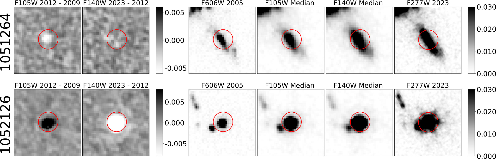
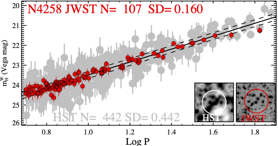
Comparison of the Hubble and JWST period and magnitude data for Cepheid variable stars in the galaxy NGC 4258. The JWST data are visibly less noisy. The inset images at the lower right show the degree of stellar crowding in the Hubble data. [Adapted from Riess et al. 2024]

A team led by Adam Riess (Space Telescope Science Institute and Johns Hopkins University) used JWST to measure the pulsation period and brightness of more than a thousand Cepheid variable stars, yielding precise measurements of the distances to these stars. This analysis showed that while the Hubble measurements are noisier than the JWST measurements, they’re no less accurate. The team ruled out at a significance of 8.2σ the possibility that inaccurate measurements of Cepheids in distant, crowded galaxies are responsible for the Hubble tension.

What If Our Assumptions Are Incorrect?

In addition to using Cepheid variable stars, many estimates of the Hubble constant rely on measurements of Type Ia supernovae, which occur when the remnant core of a low- to intermediate-mass star — a white dwarf — attains a mass of roughly 1.4 solar masses and explodes. The peak brightness of a Type Ia supernova greatly outshines a Cepheid variable, extending the cosmic distance scale out to more than a billion light-years.

plot of Hubble constant values and nonrelativistic matter density parameters calculated using different priors for the Type Ia supernova absolute magnitude

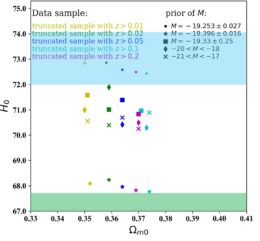
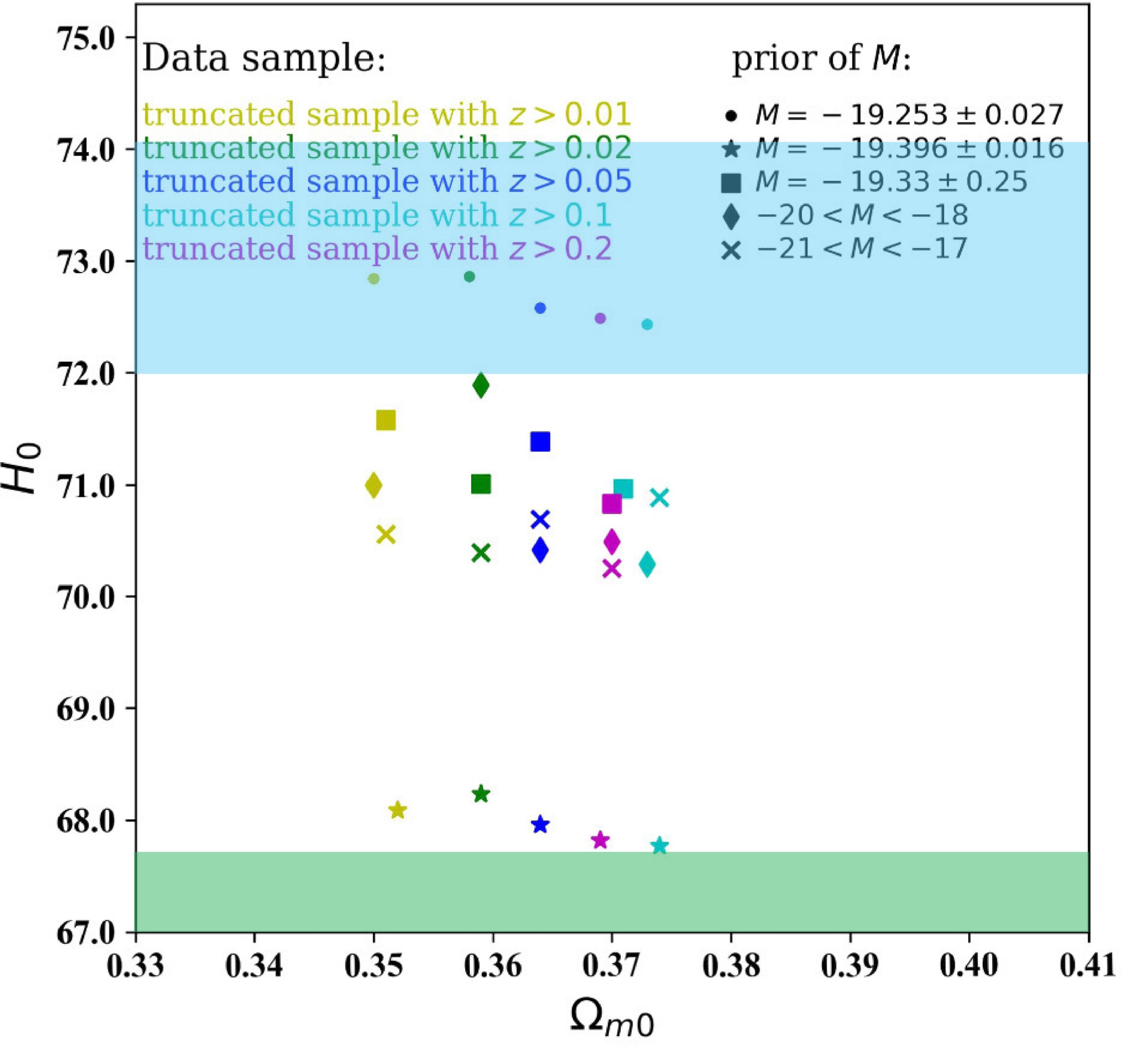
Derived values of the local-universe Hubble constant, H0, for different Type Ia supernova magnitude priors and redshift cutoffs. The blue and green shaded areas show the approximate values of the expansion measured in the local universe and extrapolated from Planck data, respectively. While the choice of supernova luminosity distribution affects the derived Hubble constant, it has little effect on Ωm0, which relates to the density of matter in the universe. See original figure set for error bars. [Adapted from Chen et al. 2024]

Because Type Ia supernovae are theorized to occur at the same limiting mass, these explosions were thought to all have the same maximum luminosity, allowing us to use them for reliable distance measurements. However, there is now evidence that not all Type Ia supernovae have the same brightness. Some are brighter than average, which may result from the collision of two white dwarfs. Some are fainter than average, which may happen when the crust of a white dwarf with a mass less than 1.4 solar masses ignites, triggering the explosion of the entire star. Other factors, like the local abundance of elements heavier than helium, might moderate a supernova’s maximum luminosity as well.

This means that instead of being limited to a single value, the maximum luminosities of Type Ia supernovae follow a distribution that is not yet well known. Yun Chen (Chinese Academy of Sciences) and collaborators examined the impact of different Type Ia supernova luminosity distributions on estimates of the Hubble constant. The team tested five luminosity distributions, three of which are Gaussians and two of which are “top hats”: equal likelihood within a certain range of luminosities and zero chance outside that range. The result? Wide-ranging values of the Hubble constant, some of which agree with the early-universe value and others of which agree with the present-day value. Given the huge impact of the underlying luminosity distribution, Chen’s team calls for a better understanding of the intrinsic properties of Type Ia supernovae.

What If We Use Another Measurement Technique?

Southern Ring Nebula from JWST

A view of the Southern Ring Nebula from JWST. [NASA, ESA, CSA, STScI]

The quest to measure the Hubble constant benefits from trying a variety of measurement techniques, and 
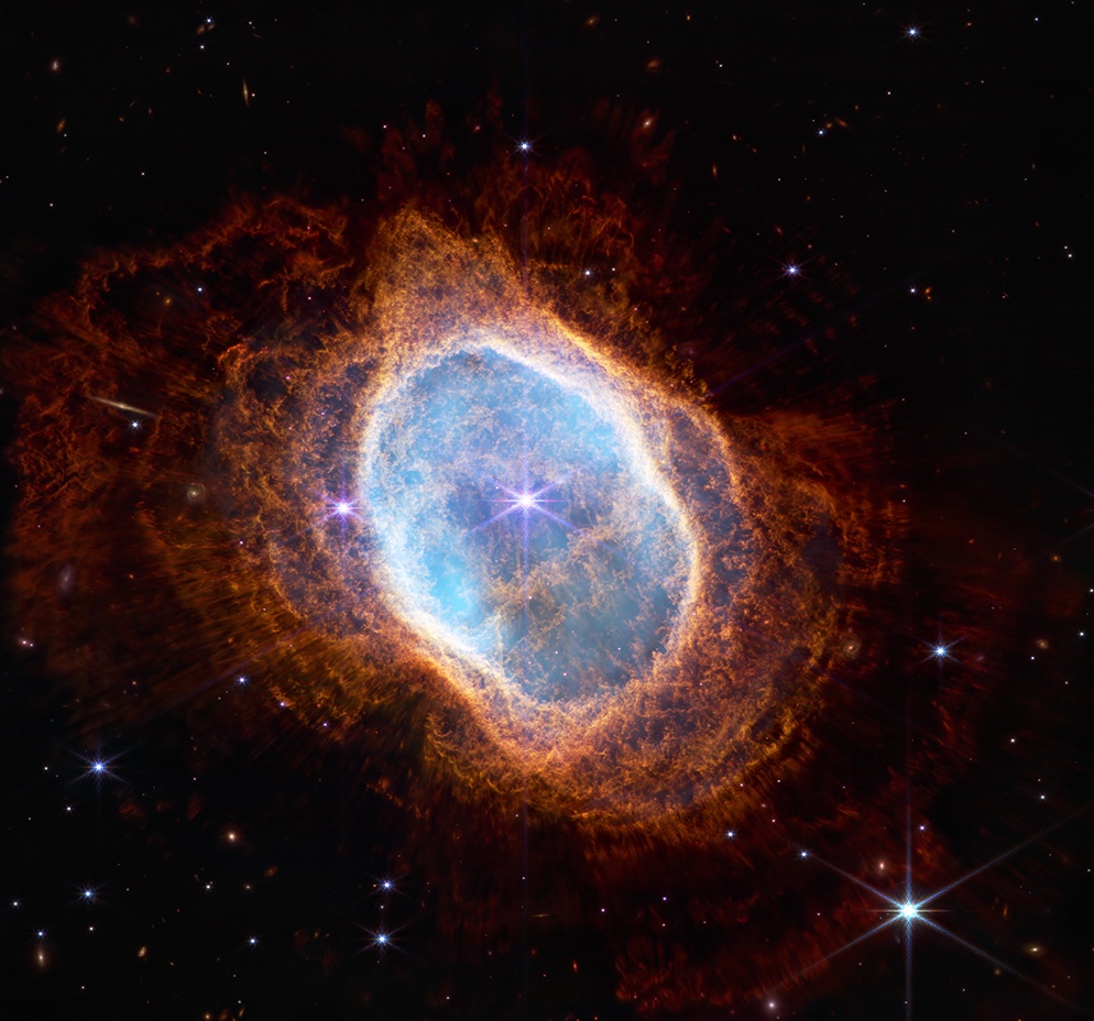
George Jacoby (NSF’s NOIRLab) and collaborators have demonstrated a unique way to measure the Hubble constant: using observations of planetary nebulae. Planetary nebulae form when stars similar in mass to the Sun — up to about 8 solar masses — lose their atmospheres at the end of their lives. High-energy photons from the exposed stellar core ionize the expelled atmospheric gas, creating a beautiful but short-lived nebula.

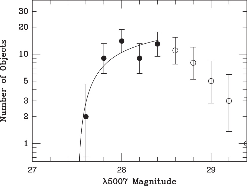
Individual planetary nebulae can have a wide range of luminosities; we can’t use single planetary nebulae to measure the distance to another galaxy as we can with Cepheid variable stars or Type Ia supernovae. However, when looking at all of the planetary nebulae in a galaxy, a remarkably consistent pattern emerges: for the brightest planetary nebulae, the number of nebulae as a function of luminosity has the same shape regardless of the properties of the galaxy in question. Using this method, researchers can measure the distances to galaxies out to about 130 million light-years.

planetary nebula luminosity function

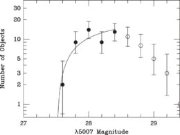
The planetary nebula luminosity function for NGC 1385. [Jacoby et al. 2024]

Jacoby’s team used archival data from the Very Large Telescope to measure the planetary nebula luminosity function for 16 galaxies. Their resulting measurement of the Hubble constant — 74.2 km/s/Mpc — is consistent with other local-universe measurements but with larger uncertainties. To measure the Hubble constant from planetary nebulae with enough precision to compare against the Type Ia supernova method, the team recommends targeted observations of a larger sample of galaxies containing at least 50 bright planetary nebulae.

What If We Could Measure the Hubble Constant from Gravitational Waves?

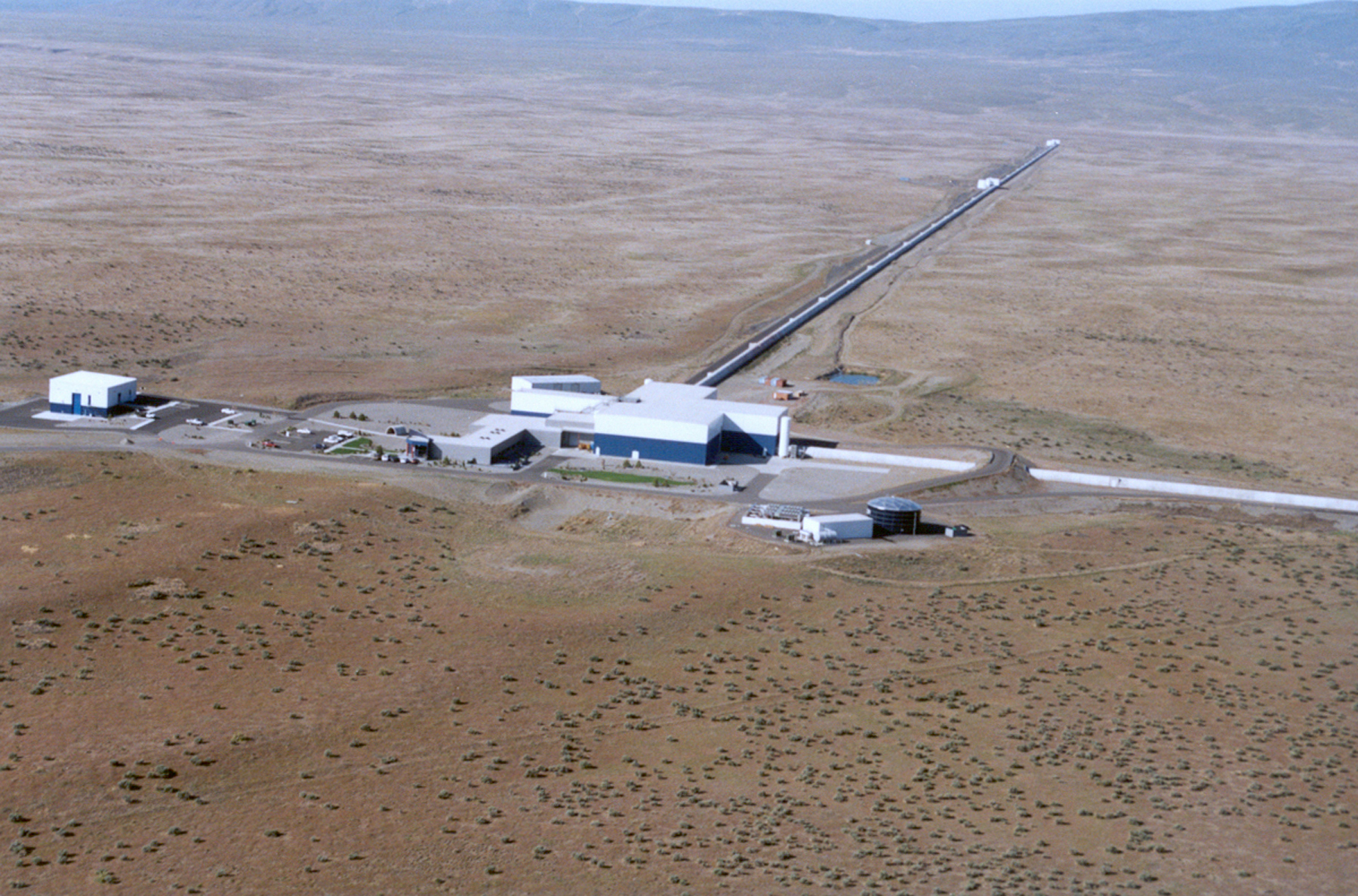
All of the Hubble-constant measurement techniques discussed so far have relied on electromagnetic radiation from one source or another. When the Laser Interferometer Gravitational-wave Observatory (LIGO) and Virgo detectors made the first direct measurement of gravitational waves in 2015, it opened a whole new window into the workings of the universe — and an entirely new way to measure its expansion rate.

Tonghua Liu (Yangtze University) and coauthors demonstrated how gravitational wave observations could enable measurements of the expansion rate out to a redshift of z = 5, or a little more than a billion years after the Big Bang. That time period is currently inaccessible to other measurement methods. Here’s how that would work: first, imagine a binary pair of neutron stars. As these objects circle one another, they expend energy in the form of gravitational waves and sink closer together, hastening their inevitable collision. As the universe expands, the expansion imprints a phase shift in the gravitational waves from the neutron star pair. This effect is tiny, amounting to just a one-second phase shift over 10 years of monitoring a neutron star binary at a redshift of z = 1. Tiny — but not impossible for future gravitational wave observatories to measure!

The phase shift and redshift of a single neutron star binary provide a direct measurement of the expansion rate of the universe at the binary system’s redshift. By measuring phase shifts for a large sample of neutron star systems across a wide range of redshifts, astronomers could measure how the expansion rate of the universe changes across cosmic time — without invoking any assumptions from a particular cosmological model.

plot of simulated acceleration parameters as a function of redshift

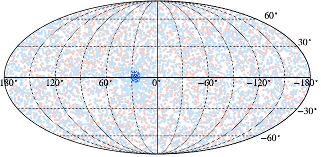
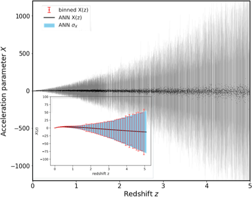
Acceleration parameters from simulated DECIGO data. After collecting a large sample of individual acceleration parameter measurements, a machine-learning algorithm can piece together the underlying trend that best fits the observations. [Liu et al. 2024]

Liu’s team simulated phase-shift measurements from a proposed space-based observatory, the Deci-hertz Interferometer Gravitational-wave Observatory (DECIGO), which is designed to detect the low-frequency gravitational waves produced by neutron star binaries years before they merge. Researchers expect that DECIGO will detect a million neutron star binaries, about 10,000 of which would be accompanied by a detectable electromagnetic signal that allows for an estimate of the binary’s redshift. Liu’s team showed that the expansion rate could be measured to within less than a percent, providing a valuable comparison to existing estimates. In addition to measuring the expansion rate, this method also yields a measurement of the universe’s curvature.

What If Dark Energy Is Responsible?

The universe is a mysterious place: according to the leading theory of cosmology, the matter that we see and interact with every day makes up just a tiny fraction — about 5% — of the contents of the universe. Dark matter, a hypothetical form of matter that interacts with everyday matter only through gravity, makes up another 27%. The majority of the matter–energy density of our universe comes from the most mysterious quantity of all: dark energy. Dark energy is thought to provide the outward pressure responsible for the accelerating expansion of the universe, but the exact cause of this pressure remains unknown.

probability distribution function for values of the hubble constant for different models of oscillating dark matter

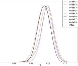
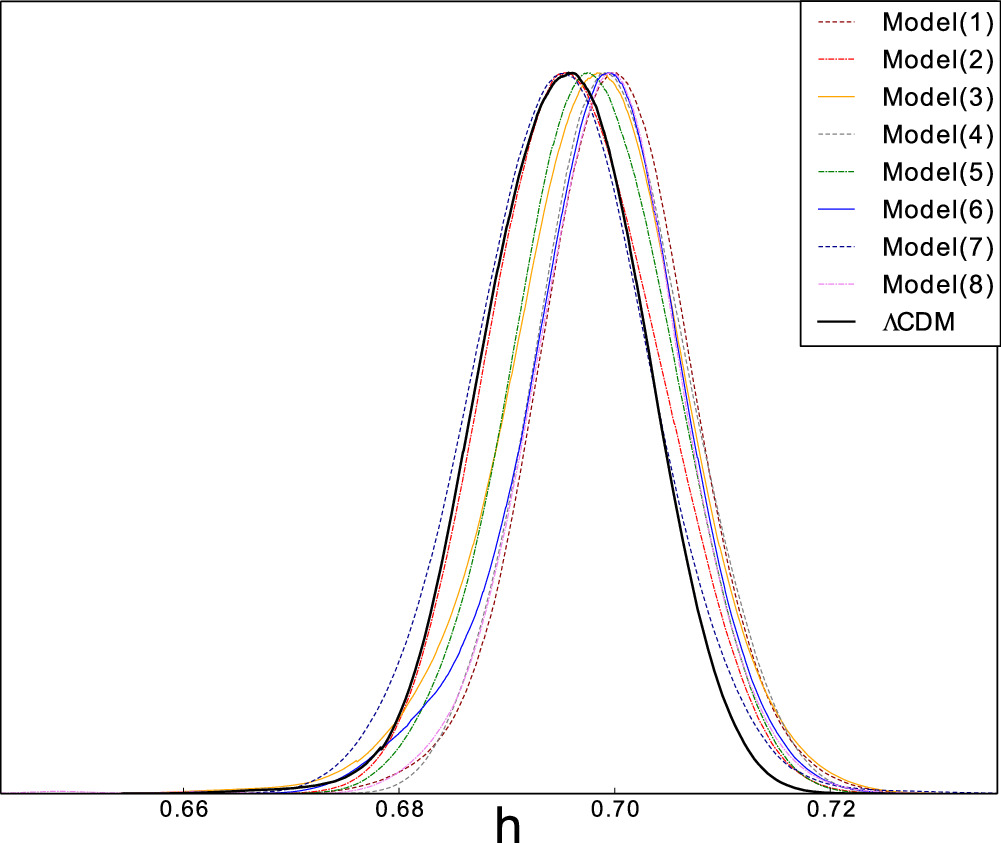
Probability distribution of the expansion rate (shown here as the rate divided by 100) for different descriptions of oscillating dark matter. The black line shows the result from ΛCDM for comparison. [Rezaei 2024]

The persistence of the Hubble tension has led some researchers to propose alternative theories of cosmology, many of which adjust the properties and identities of dark matter and dark energy. Recently, Mehdi Rezaei (Hamedan Research Center for Applied Meteorology) investigated the impact of oscillating dark energy on the Hubble tension. If dark energy were to oscillate between accelerating and decelerating the expansion of the universe at different points in cosmic time, it could explain the mismatch between the extrapolated early-universe expansion rate and the present-day rate. Using eight different descriptions of oscillating dark energy that have been presented in previous research, Rezaei found that these prescriptions reduced the Hubble tension from its current 5σ severity to 2.14–2.56σ.

In addition to making progress on the Hubble tension, oscillating dark matter could solve another problem of cosmological importance called the coincidence problem. Essentially, the coincidence problem boils down to the fact that in the present-day universe the energy densities of dark matter and dark energy are of the same order of magnitude — but in the distant past and distant future these quantities were/will be way out of balance. In the oscillating dark energy scenario, the energy densities of dark matter and dark energy ebb and flow, and they would have been equal at several points in the universe’s history. While oscillating dark energy alleviates the Hubble tension and the coincidence problem, it doesn’t fit certain observations as well as ΛCDM does — and the search for a definitive solution to the Hubble tension goes on!

Citation

“JWST Observations Reject Unrecognized Crowding of Cepheid Photometry as an Explanation for the Hubble Tension at 8σ Confidence,” Adam G. Riess et al 2024 ApJL 962 L17. doi:10.3847/2041-8213/ad1ddd

“Effects of Type Ia Supernovae Absolute Magnitude Priors on the Hubble Constant Value,” Yun Chen et al 2024 ApJL 964 L4. doi:10.3847/2041-8213/ad2e97

“Toward Precision Cosmology with Improved Planetary Nebula Luminosity Function Distances Using VLT-MUSE. II. A Test Sample from Archival Data,” George H. Jacoby et al 2024 ApJS 271 40. doi:10.3847/1538-4365/ad2166

“Model-Independent Way to Determine the Hubble Constant and the Curvature from the Phase Shift of Gravitational Waves with DECIGO,” Tonghua Liu et al 2024 ApJL 965 L11. doi:10.3847/2041-8213/ad3553

“Oscillating Dark Energy in Light of the Latest Observations and Its Impact on the Hubble Tension,” Mehdi Rezaei 2024 ApJ 967 2. doi:10.3847/1538-4357/ad3963

illustration of two neutron stars spiraling toward each other

In May of last year, an international collaboration of astronomers and physicists switched on a set of detectors and began the most intensive search for gravitational waves ever attempted. They did not have to wait long for a new discovery that challenges our understanding of the extreme universe: just days into their campaign, the scientists caught the signal from the smallest black hole ever detected by their observatories, one that is so light it couldn’t have formed according to our typical models. After a year of analysis, the scores of scientists involved in this remarkable find have just published their work in The Astrophysical Journal Letters.

How To Warp Spacetime

Although gravitational waves, or ripples in spacetime caused by collisions between massive objects, have permeated the universe since its very beginning, scientists have only been able to directly measure them since 2015. Since then, we’ve learned much about these waves and the objects that source them, and we’ve built up a pretty clear picture of what it takes to wrinkle space itself.

photograph of the LIGO Hanford gravitational wave detector

A gravitational wave detector. Ripples in spacetime cause the two arms to change lengths by tiny amounts, and scientists detect passing waves by carefully measuring these distortions. [Caltech/MIT/LIGO Lab]

In short, you need a pair of enormously heavy objects to smash into each other at high speeds. Two types of objects will do the trick: neutron stars, or the exotic remains of supernova explosions, and the more massive and more infamous black holes.

Neutron stars, as best we understand from theoretical models and observations taken with radio and X-ray telescopes, can weigh up to about 3 times the mass of the Sun and are formed when a large star explodes. Black holes, on the other hand, are typically heavier. They weigh more than 5 times the mass of the Sun, and they’re thought to form when a large star collapses in on itself.

Putting these two facts together, it’d be very strange to identify an object that’s between 3 and 5 solar masses: anything in that gap would be too heavy to be a neutron star, but too light to be a black hole. And yet, that’s exactly what the international collaboration found: the collision between a 1.4-solar-mass neutron star and a 3.6-solar-mass black hole, making the latter an inhabitant of the so-called “mass gap.”

A Rule-Breaking Merger

The inferred masses of each component of a handful of gravitational wave mergers. The “mass gap” is marked in light grey, and the likely mass of the primary component of this event, GW230529, lies nearly entirely within it. [A. G. Abac et al 2024]

Their merger, named in the traditionally catchy parlance of astronomers as GW230529_181500, was a real surprise. Though the collaboration has a total of four gravitational wave detectors at its disposal, only one saw the signal: the newest, named KAGRA, is not sensitive enough to spot an event this faint, while VIRGO was undergoing upgrades at the time and one of the two LIGO sites had been switched off only an hour and a half too soon to catch the show. This lack of detector backup, combined with the weirdness of the implied progenitor, left the team with a lot of work to do to prove that what they were seeing was real.

In the end, the event passed all of their tests. The wave was detected by three independent analysis pipelines, and although the choices that go into modeling the collision can affect the inferred mass, most reasonable options all point to the same conclusion: the observed gravitational wave really does seem to have come from an impossibly light black hole and its merger with a typical neutron star. This proof-by-contradiction that small black holes exist implies that there are probably plenty of them, which happily means we can look forward to additional head-scratching detections of similar pairs in the future.

Citation

“Observation of Gravitational Waves from the Coalescence of a 2.5–4.5 M⊙ Compact Object and a Neutron Star,” A. G. Abac et al 2024 ApJL 970 L34. doi:10.3847/2041-8213/ad5beb

Hubble image of the Flame Nebula

visualization of a turbulent flow

Visualization of the plume from a candle transitioning from a smooth flow near the wick to a turbulent flow higher up. [Gary Settles; CC BY-SA 3.0]

Turbulence — the culprit behind bumpy airplane rides, breaking waves, and billowing clouds — happens throughout the universe. Modeling realistic turbulent plasmas is difficult and computationally expensive, but new methods make simulating turbulence easier, faster, and more flexible than ever before.

A Chaotic Challenge

In the accretion disks around supermassive black holes, the clouds of molecular gas where stars are born, and even the atmosphere of the Sun, turbulence plays an important role in transferring energy and mixing plasmas. Because turbulent plasmas are so common, researchers across astronomical fields must wrestle with the challenge of modeling these chaotic systems.

The traditional way to model a turbulent system is to do so numerically: churning through sets of equations to track the behavior of a plasma across tiny time increments. But as models become more complex, this comes at a higher computational cost, requiring an increasingly large number of hours for computers to handle the math.

representation of a simulated three-dimensional turbulent magnetic field

A representation of a typical three-dimensional turbulent magnetic field generated by BxC. [Adapted from Maci et al. 2024]

Synthetic Magnetic Fields

Synthetic models that use relatively simple algorithms to generate realistic plasmas provide an alternative. Recently, Daniela Maci (KU Leuven) and collaborators introduced a new synthetic model of turbulent magnetic fields. The team’s model builds on an existing synthetic model called BxC, a Python-based code that speedily produces three-dimensional turbulent magnetic fields.

To generate realistic turbulence, BxC starts with a random field of vectors based on white noise. From there, this vector field is tweaked and transformed to adjust its statistical properties. In practice, this means that not only do BxC’s synthetic fields look turbulent, they also reproduce the expected statistical properties of a turbulent field, setting BxC apart from other models. This makes BxC an excellent jumping-off platform for creating realistic turbulent magnetic fields, and Maci’s team showed how the statistical properties of the modeled field depend on the model’s inputs.

Paths Forward

simulation results showing turbulence that develops on top of a background magnetic field

Examples of simulated turbulence that develops on top of a background magnetic field. Click to enlarge. [Adapted from Maci et al. 2024]

To make the synthetic fields more applicable to astrophysical plasmas, Maci’s team expanded upon the original code in a couple of key ways. First, they recognized that turbulence often develops on top of a background magnetic field, and they developed a way for turbulence to be applied while maintaining the underlying structure of the field. This applies to magnetic field structures like loops or flux tubes, both of which are seen in the atmosphere of the Sun. Second, they developed a way to incorporate anisotropy, or a difference in the strength of the turbulence with regard to direction.

This work demonstrates the power and flexibility of synthetic models for representing turbulent magnetic fields — and all of these features are available orders of magnitude faster than they would be from a traditional numerical model. The team anticipates making future additions to their model, all of which would give the user more customization options and make the model applicable to more astrophysical scenarios.

Citation

“BxC Toolkit: Generating Tailored Turbulent 3D Magnetic Fields,” Daniela Maci et al 2024 ApJS 273 11. doi:10.3847/1538-4365/ad4bdf

1 11 12 13 14 15 112