Features RSS

Kilonova

Bitten by the gravitational-wave bug? While we await Thursday’s press conference, here’s some food for thought: if LIGO were able to detect gravitational waves from compact-object mergers, how could we follow up on the detections? A new study investigates whether the upcoming James Webb Space Telescope (JWST) will be able to observe electromagnetic signatures of some compact-object mergers.

Hunting for Mergers

Studying compact-object mergers (mergers of black holes and neutron stars) can help us understand a wealth of subjects, like high-energy physics, how matter behaves at nuclear densities, how stars evolve, and how heavy elements in the universe were created.

The Laser Interferometer Gravitational-Wave Observatory (LIGO) is searching for the signature ripples in spacetime identifying these mergers, but gravitational waves are squirrelly: LIGO will only be able to localize wave sources to tens of square degrees. If we want to find out more about any mergers LIGO discovers in gravitational waves, we’ll need a follow-up search for electromagnetic counterparts with other observatories.

The Kilonova Key

One possible electromagnetic counterpart is kilonovae, explosions that can be produced during a merger of a binary neutron star or a neutron star–black hole system. If the neutron star is disrupted during the merger, some of the hot mass is flung outward and shines brightly by radioactive decay.

Kilonovae are especially promising as electromagnetic counterparts to gravitational waves for three reasons:

  1. They emit isotropically, so the number of observable mergers isn’t limited by relativistic beaming.
  2. They shine for a week, giving follow-up observatories time to search for them.
  3. The source location can be easily recovered.

The only problem? We don’t currently have any sensitive survey instruments in the near-infrared band (where kilonova emission peaks) that can provide coverage over tens of square degrees. Luckily, we will soon have just the thing: JWST, launching in 2018!

JWST’s Search

NIRCam capabilities

Integration time needed for JWST’s NIRCam to detect a kilonova at 200 Mpc, as a function of time since the merger. Different curves correspond to different NIRCam filters. Note that the total time for follow-up is overwhelmingly dominated by things like telescope slew time, rather than by this exposure time. [Bartos et al. 2016]

In a recent study, a team of authors led by Imre Bartos (Columbia University) evaluate whether JWST will be capable of catching these kilonovae if LIGO finds gravitational wave signals.

Bartos and collaborators calculate that, given the sensitivity of the different filters on JWST’s Near-Infrared Camera, the instrument should easily be able to detect a kilonova 200 Mpc away (a typical distance at which LIGO might be able to find a neutron-star binary). But there’s a catch: 10 deg2 is a really big sky area, and it would take JWST an unfeasible amount of time (days!) to fully cover it.

The authors suggest instead using a targeted search. Since most mergers are expected to be in or near galaxies, JWST could specifically focus the follow-up search on known galaxies within the search area. This approach would bring the total search time down to 12.6 hours, which is within the realm of feasibility. And this time could be reduced even further by concentrating on galaxies most likely to host kilonovae, like those with high star-formation rates.

The conclusion: if LIGO is able to detect gravitational waves, JWST will provide an excellent means to follow up on the detection in the attempt to identify the source.

Citation

I. Bartos et al 2016 ApJ 816 61. doi:10.3847/0004-637X/816/2/61

Small exoplanets

Small exoplanets tend to fall into two categories: the smallest ones are predominantly rocky, like Earth, and the larger ones have a lower-density, more gaseous composition, similar to Neptune. The planet Kepler-454b was initially estimated to fall between these two groups in radius. So what is its composition?

Small-Planet Dichotomy

Though Kepler has detected thousands of planet candidates with radii between 1 and 2.7 Earth radii, we have only obtained precise mass measurements for 12 of these planets.

mass-radius relation

Mass-radius diagram (click for a closer look!) for planets with radius <2.7 Earth radii and well-measured masses. The six smallest planets (and Venus and Earth) fall along a single mass-radius curve of Earth-like composition. The six larger planets (including Kepler-454b) have lower-density compositions. [Gettel et al. 2016]

These measurements, however, show an interesting dichotomy: planets with radii less than 1.6 Earth radii have rocky, Earth-like compositions, following a single relation between their mass and radius. Planets between 2 and 2.7 Earth radii, however, have lower densities and don’t follow a single mass-radius relation. Their low densities suggest they contain a significant fraction of volatiles, likely in the form of a thick gas envelope of water, hydrogen, and/or helium.

The planet Kepler-454b, discovered transiting a Sun-like star, was initially estimated to have a radius of 1.86 Earth radii — placing it in between these two categories. A team of astronomers led by Sara Gettel (Harvard-Smithsonian Center for Astrophysics) have since followed up on the initial Kepler detection, hoping to determine the planet’s composition.

Low-Density Outcome

Gettel and collaborators obtained 63 observations of the host star’s radial velocity with the HARPS-N spectrograph on the Telescopio Nazionale Galileo, and another 36 observations with the HIRES spectrograph at Keck Observatory. These observations allowed them to do several things:

  1. Obtain a more accurate radius estimate for Kepler-454b: 2.37 Earth radii.
  2. Measure the planet’s mass: roughly 6.8 Earth masses.
  3. Discover — surprise! — two other, non-transiting companions in the system: Kepler-454c, a planet with a minimum mass of ~4.5 Jupiter masses on a 524-day orbit, and Kepler-454d, a more distant (>10-year orbit) brown dwarf or low-mass star.

Kepler-454b’s newly measured size and mass place it firmly in the category of non-rocky, larger, less dense planets (the authors calculate a density of ~2.76 g/cm3, or roughly half that of Earth). This seems to reinforce the idea that rocky planets don’t grow larger than ~1.6 Earth radii, and planets with mass greater than about 6 Earth masses are typically low-density and/or swathed in an envelope of gas.

The authors point out that future observing missions like NASA TESS (launching in 2017) will provide more targets that can be followed up to obtain mass measurements, allowing us to determine if this trend in mass and radius holds up in a larger sample.

Citation

Sara Gettel et al 2016 ApJ 816 95. doi:10.3847/0004-637X/816/2/95

Fermi 2FHL sky map

The Large Area Telescope (LAT) on board the Fermi Gamma-ray Space Telescope has received an upgrade that increased its sensitivity by a whopping 40% — and nobody had to travel to space to make it happen! The difference instead stems from remarkable improvement to the software used to analyze Fermi-LAT’s data, and it has resulted in a new high-energy map of our sky.

Pass 8 v. Pass 7

Animation (click to watch!) comparing the Pass 7 to the Pass 8 Fermi-LAT analysis, in a region in the constellation Carina. Pass 8 provides more accurate directions for incoming gamma rays, so more of them fall closer to their sources, creating taller spikes and a sharper image. [NASA/DOE/Fermi LAT Collaboration]

Pass 8

Fermi-LAT has been surveying the whole sky since August 2008. It detects gamma-ray photons by converting them into electron-positron pairs and tracking the paths of these charged particles. But differentiating this signal from the charged cosmic rays that also pass through the detector — with a flux that can be 10,000 times larger! — is a challenging process. Making this distinction and rebuilding the path of the original gamma ray relies on complex analysis software.

“Pass 8” is a complete reprocessing of all data collected by Fermi-LAT. The software has gone through many revisions before now, but this is the first revision that has taken into account all of the experience that the Fermi team has gained operating the LAT in its orbital environment.

The improvements made in Pass 8 include better background rejection of misclassified charged particles, improvements to the point spread function and effective area of the detector, and an extension of the effective energy range from below 100 MeV to beyond a few hundred GeV. The changes made in Pass 8 have increased the sensitivity of Fermi-LAT by an astonishing 40%.

Map of the High-Energy Sky

2FHL sources

Sky map of the sources in the 2FHL catalog, classified by their most likely association. Click for a better look! [Ackermann et al. 2016]

The first result from the improvements of Pass 8 is 2FHL, the second catalog of high-energy Fermi sources, constructed from 80 months of data from Fermi-LAT.  The 2FHL catalog contains 360 sources from across the sky in the 50 GeV–2TeV range. Here are just a few details:

  • 47 of the sources are new — they have not previously been detected by Fermi or ground-based gamma-ray detectors.
  • 86% of the sources can be associated with counterparts at other wavelengths. This includes
    • 75% that are active galactic nuclei, and
    • 11% that originate in our galaxy, the majority of which are associated with objects at the final stage of stellar evolution, such as pulsar wind nebulae and supernova remnants.

Because the quality of Fermi-LAT’s observations is limited by the number of photons collected, longer observing time will only serve to improve the detections in this catalog. And since only 22% of the 2FHL sources have been observed by ground-based gamma-ray detectors (which have much more limited fields of view), this catalog provides an excellent list of candidates that these detectors can now follow up at very high energies.

Bonus

Want to learn more about Pass 8? Check out this video, created by the Fermi team. [NASA’s Goddard Space Flight Center]

Citation

M. Ackermann et al 2016 ApJS 222 5. doi:10.3847/0067-0049/222/1/5

Saturn and Titan

Have you ever wondered what springtime is like on Saturn’s largest moon, Titan? A team of researchers has analyzed a decade of data from the Cassini spacecraft to determine how Titan’s gradual progression through seasons has affected its temperatures.

Observing the Saturn System

Though Titan orbits Saturn once every ~16 days, it is Saturn’s ~30-year march around the Sun that sets Titan’s seasons: each traditional season on Titan spans roughly 7.5 years. Thus, when the Cassini spacecraft first arrived at Saturn in 2004 to study the giant planet and its ring system and moons, Titan’s northern hemisphere was in early winter. A decade later, the season in the northern hemisphere had advanced to late spring.

A team scientists led by Donald Jennings (Goddard Space Flight Center) has now used data from the Composite Infrared Spectrometer (CIRS) on board Cassini to analyze the evolution of Titan’s surface temperature between 2004 and 2014.

Changing of Seasons

Titan surface temperatures

Surface brightness temperatures (with errors) on Titan are shown in blue for five time periods between 2004 and 2014. The location of maximum temperature migrates from 19°S to 16°N over the decade. Two climate models are also shown in green (high thermal inertia) and red (low thermal inertia). [Jennings et al. 2016]

CIRS uses the decreased opacity of Titan’s atmosphere at 19 µm to detect infrared emission from Titan’s surface at this wavelength. From this data, Jennings and collaborators determine Titan’s surface temperature for five time intervals between 2004 and 2014. They bin the data into 10° latitude bins that span from the south pole (90°S) to the north pole (90°N).

The authors find that the maximum temperature on the moon stays stable over the ten-year period at 94 K, or a chilly -240°F). But as time passes, the latitude with the warmest temperature shifts from 19°S to 16°N, marking the transition from early winter to late spring. Over the decade of monitoring, the surface temperature near the south pole decreased by ~2 K, and that near the north pole increased by ~1 K.

Climate Modeling

Though Titan’s overall temperature trend is expected, the rate of change of its surface temperature doesn’t quite match theoretical climate models: the northern hemisphere lags slightly behind the predicted temperature curve. The authors speculate that this may be due to the effects of seas in Titan’s northern hemisphere. Seas of hydrocarbons (e.g., methane) are thought to account for ~10% of the moon’s surface area at latitudes of 55–90°N. Since the seas have a higher thermal inertia than land, this could explain why temperatures in Titan’s northern hemisphere lag behind the model’s predictions.

The authors hope to gain additional data in the future, as CIRS has another two years of operation planned before the Cassini mission ends. This time span will take us all the way up to Titan’s northern summer solstice; it will be exciting to see what more we can learn from this data!

Citation

D. E. Jennings et al 2016 ApJ 816 L17. doi:10.3847/2041-8205/816/1/L17

X-ray jet

Accreting, supermassive black holes that reside at galactic centers can power enormous jets, bright enough to be observed from vast distances away. The recent discovery of such a jet in X-ray wavelengths, without an apparent radio counterpart, has interesting implications for our understanding of how these distant behemoths shine.

An Excess of X-Rays

Quasar B3 0727+409 was serendipitously discovered to host an X-ray jet when a group of scientists, led by Aurora Simionescu (Institute of Space and Astronautical Sciences of the Japan Aerospace Exploration Agency), was examining Chandra observations of another object.

The Chandra data reveal bright, compact, extended emission from the core of quasar B3 0727+409, with a projected length of ~100 kpc. There also appears to be further X-ray emission at a distance of ~280 kpc, which Simionescu and collaborators speculate may be the terminal hotspot of the jet.

The quasar is located at a redshift of z=2.5 — which makes this jet one of only a few high-redshift X-ray jets known to date. But what makes it especially intriguing is that, though the authors searched through both recent and archival radio observations of the quasar, the only radio counterpart they could find was a small feature close to the quasar core (which may be a knot in the jet). Unlike what is typical of quasar jets, there was no significant additional radio emission coinciding with the rest of the X-ray jet.

Making Jets Shine

Inverse-Compton CMB models

X-ray-to-radio flux ratio vs. redshift, for X-ray quasar jets detected with Chandra. B3 0727+409 is shown in red (with and without the radio knot). The curves represent inverse-Compton scattering models with different magnetic field strengths. [Simionescu et al. 2016]

What does this mean? To answer this, we must consider one of the outstanding questions about quasar jets: what radiation processes dominate their emission? One process possibly contributing to the X-ray emission is inverse-Compton scattering of low-energy cosmic microwave background (CMB) photons off of the electrons in the jet; these photons can scatter up to X-ray energies.

Interestingly, there’s a testable prediction associated with this mechanism. If this process dominates the X-ray emission of quasar jets, then the X-ray-to-radio flux ratio of the jet would increase with redshift as (1+z)4, due to the increased density of CMB photons at higher redshift.

Thus far, our limited detections of high-redshift X-ray quasars have made it difficult to test this prediction, but quasar B3 0727+409 provides an extremely useful data point. When the authors model the radio-to-X-ray flux ratio for the jet, they find that it’s entirely consistent with the inverse-Compton scenario.

This discovery suggests that the inverse-Compton mechanism may indeed be what dominates the X-ray radiation from jets like this one. And since our current observing strategies focus on Chandra follow-up of known bright radio jets, this could mean that there is an entire population of similar systems — with bright X-ray and faint radio emission — that we have missed!

Citation

A. Simionescu et al 2016 ApJ 816 L15. doi:10.3847/2041-8205/816/1/L15

binary companion

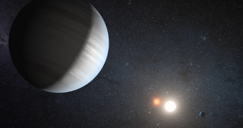
The Friends of Hot Jupiters (FOHJ) project is a systematic search for planetary- and stellar-mass companions in systems that have known hot Jupiters — short-period, gas-giant planets. This survey has discovered that many more hot Jupiters may have companions than originally believed.

Missing Friends

FOHJ was begun with the goal of better understanding the systems that host hot Jupiters, in order to settle several longstanding issues.

The first problem was one of observational statistics. We know that roughly half of the Sun-like stars nearby are in binary systems, yet we’ve only discovered a handful of hot Jupiters around binaries. Are binary systems less likely to host hot Jupiters? Or have we just missed the binary companions in the hot-Jupiter-hosting systems we’ve seen so far?

An additional issue relates to formation mechanisms. Hot Jupiters probably migrated inward from where they formed out beyond the ice lines in protoplanetary disks — but how?

AO image

This median-stacked image, obtained with adaptive optics, shows one of the newly-discovered stellar companions to a star hosting a hot Jupiter. The projected separation is ~180 AU. [Ngo et al. 2015]

Observations reveal two populations of hot Jupiters: those with circular orbits aligned with their hosts’ spins, and those with eccentric, misaligned orbits. The former population support a migration model dominated by local planet-disk interactions, whereas the latter population suggest the hot Jupiters migrated through dynamical interactions with distant companions. A careful determination of the companion rate in hot-Jupiter-hosting systems could help establish the ability of these two models to explain the observed populations.

Search for Companions

The FOHJ project began in 2012 and studied 51 systems hosting known, transiting hot Jupiters — with roughly half on circular, aligned orbits and half on eccentric, misaligned orbits. The survey consisted of three different, complementary components:

  • Study 1
    Lead author: Heather Knutson (Caltech)
    Technique: Long-term radial velocity monitoring
    Searching for: Planetary companions at 1–20 AU from the star
  • Study 2
    Lead author: Henry Ngo (Caltech)
    Technique: Adaptive-optics imaging
    Searching for: Stellar companions at 50–2000 AU from the star
  • Study 3
    Lead author: Danielle Piskorz (Caltech)
    Technique: Spectroscopy
    Searching for: Any additional stellar companions at <125 AU from the star
binary fractions

The companion fraction found within Study 2, the adaptive-optics imagine search. The three curves show the total, the systems with hot Jupiters on aligned and circular orbits, and those with hot Jupiters on misaligned and eccentric orbits. [Ngo et al. 2015]

Migration Implications

Using these three different techniques, the team found a significant number of both planetary and stellar companions that had not been previously detected. After correcting their results for completeness, they found a multiple-star rate of ~50% for these systems, resolving the problem of the missing companions. So really, we just weren’t looking hard enough for the companions previously.

Intriguingly, the binary companion rate found for these hot Jupiter systems is higher than the average rate for the field stars (which is below 25% for the semimajor-axis range the FOHJ studies are sensitive to). This suggests that companion stars may indeed play a role in hot Jupiter formation and migration.

That said, none of the three studies found a significant difference in the binary fraction for aligned versus misaligned hot Jupiters — which means that the answer is not as simple as thought, with companion stars causing the misaligned planets. Thus, while hot Jupiters’ “friends” may play a role in their formation and migration, we still have work to do in understanding what that role is.

Citation

Danielle Piskorz et al 2015 ApJ 814 148. doi:10.1088/0004-637X/814/2/148
Henry Ngo et al 2015 ApJ 800 138. doi:10.1088/0004-637X/800/2/138
Heather A. Knutson et al 2014 ApJ 785 126. doi:10.1088/0004-637X/785/2/126

Ophiuchus stream's orbit

Dwarf galaxies or globular clusters orbiting the Milky Way can be pulled apart by tidal forces, leaving behind a trail of stars known as a “stellar stream.” One such trail, the Ophiuchus stream, has posed a serious dynamical puzzle since its discovery. But a recent study has identified four stars that might help resolve this stream’s mystery.

Conflicting Timescales

The stellar stream Ophiuchus was discovered around our galaxy in 2014. Based on its length, which appears to be 1.6 kpc, we can calculate the time that has passed since its progenitor was disrupted and the stream was created: ~250 Myr. But the stars within it are ~12 Gyr old, and the stream orbits the galaxy with a period of ~350 Myr.

Given these numbers, we can assume that Ophiuchus’s progenitor completed many orbits of the Milky Way in its lifetime. So why would it only have been disrupted 250 million years ago?

Fanning Stream

Led by Branimir Sesar (Max Planck Institute for Astronomy), a team of scientists has proposed an idea that might help solve this puzzle. If the Ophiuchus stellar stream is on a chaotic orbit — common in triaxial potentials, which the Milky Way’s may be — then the stream ends can fan out, with stars spreading in position and velocity.

The fanned part of the stream, however, would be difficult to detect because of its low surface brightness. As a result, the Ophiuchus stellar stream could actually be longer than originally measured, implying that it was disrupted longer ago than was believed.

Search for Fan Stars

To test this idea, Sesar and collaborators performed a search around the ends of the stream, looking for stars that

  1. are of the right type to match the stream,
  2. are at the predicted distance of the stream,
  3. are located near the stream ends, and
  4. have velocities that match the stream and don’t match the background halo stars.
Target star velocities

Histogram of the heliocentric velocities of the 43 target stars. Six stars have velocities matching the stream velocity. Two of these are located in the main stream; the other four may be part of a fan at the end of the stream. [Sesar et al. 2016]

Of the 43 targets for which the authors obtained spectra, four stars met these criteria and are located beyond the main extent of the stream, possibly comprising a fan at the stream’s end. Including these stars as part of the Ophiuchus stream, its length becomes 3 kpc, implying that its time of disruption was closer to 400 million years ago. This relieves the timescale tension but does not resolve it.

That said, the mere evidence of a fan in the Ophiuchus stream suggests that its progenitor may have been on a chaotic orbit. If this is the case, it’s entirely possible that the progenitor could have survived for ~11 Gyr, only to have been disrupted within the last 0.5 Gyr. Detailed modeling and further identification of potential fan stars in the Ophiuchus stream will help to test this idea and resolve the puzzle of this stream.

Citation

Branimir Sesar et al 2016 ApJ 816 L4. doi:10.3847/2041-8205/816/1/L4

Planet Nine

The recent discovery that the orbits of some Kuiper belt objects (KBOs) share properties has proved puzzling. A pair of scientists have now proposed a bold explanation: there may be a planet-sized object yet undetected in our solar system.

Mysterious Clustering

KBOs, the population of mainly small objects beyond Neptune, have proven an especially interesting subject of study in the last decade as many small, distant bodies (such as Eris, the object that led to the demotion of Pluto to dwarf planet) have been discovered.

Previous studies have recently discovered that some especially distant KBOs — those that orbit with semimajor axes of a > 150 AU, nearly four times that of Pluto — all cross the ecliptic at a similar phase in their elliptical trajectories. This is unexpected, since gravitational tugs from the giant planets should have randomized this parameter over our solar system’s multi-billion-year lifespan.

Physical alignment of the orbits of Kuiper belt objects with a > 250 AU (and two objects with a > 150 AU that are dynamically stable). [Batygin & Brown 2016]

Physical alignment of the orbits of Kuiper belt objects with a > 250 AU (and two objects with a > 150 AU that are dynamically stable). [Batygin & Brown 2016]

Two scientists at California Institute of Technology, Konstantin Batygin and Michael Brown (you might recognize Brown as the man who “killed Pluto”) have now increased the mystery. In a recently published a study, they demonstrate that for KBOs that have orbits with a > 250 AU, the orbits are actually physically aligned.

To explain this unexpected alignment — which Batygin and Brown calculate has only a 0.007% probability of having occurred by chance — the authors ask an exciting question: could this be caused by the presence of an unseen, large, perturbing body further out in the solar system?

Simulating a Ninth Planet

The authors test this hypothesis by carrying out both analytical calculations and numerical N-body simulations designed to determine if the gravitational influence of a distant, planetary-mass companion can explain the behavior we observe from the large-orbit KBOs.

Simulation of Planet Nine's effects

Simulation of the effect of a distant planet (M = 10 M, a = 700 AU, and e = 0.6) on KBOs; click for a better look! The perihelion position of KBOs with a > 250 AU clusters around 180° from the perihelion position of the perturbing planet. More-transparent points are less observable. [Batygin & Brown 2016]

The result? It turns out that such a distant planet can cause the orbits of KBOs with a > 250 AU to all align in the opposite direction of the orbit of the planet. What’s more, the gravitational pull of this planet can also explain other unresolved puzzles about the Kuiper belt, such as the presence of high-perihelion Sedna-like objects, as well as a population of KBOs we’ve observed that have misaligned orbits.

Unfortunately, Batygin and Brown found it isn’t possible to exactly determine the properties of the possible planet, since multiple combinations of its mass, eccentricity, and semimajor axis can create the same observational results. That said, they believe the distant perturber’s orbit is highly eccentric, its orbital inclination is low, and it’s fairly massive (since anything less than an Earth-mass won’t create the observed clustering of KBO orbits within the age of the solar system).

As an example, one possible set of parameters that approximately reproduces the observed KBO orbits is the following:

  • planet mass of 10 Earth-masses
  • semi-major axis of a = 700 AU
  • eccentricity of e = 0.6

This would correspond to a perihelion distance of 280 AU and an aphelion distance of 1,120 AU.

The authors speculate such a planet might have been formed closer in to the Sun, but it was ejected later on during our solar system’s evolution. Interactions with the Sun’s birth cluster could have then caused the planet to be retained in a bound orbit.

Future Tests

Solar system

Our solar system on a logarithmic scale (click for the full view). KBOs with a semimajor axis of a > 250 AU may be being aligned by a planetary-mass body with an even more distant orbit. [NASA]

How can we test this hypothesis of a ninth planet? Obviously, directly observing the planet would confirm its presence. But the authors’ model has an additional testable hypothesis: if it’s correct, there should be a population of high-perihelion Kuiper belt objects that don’t exhibit the same alignment of their orbits as the KBOs we know about, but instead have opposite-aligned orbits. If we discover such a collection of objects, that would be an excellent confirmation of this model.

The authors caution that their work is preliminary, and additional investigation will be required to better understand the possibilities presented here. But with any luck, future theoretical work, as well as observational tests of this model’s predictions, will help us determine whether there might be a distant ninth planet in our solar system!

Bonus

Check out this video (created with WWT!), which walks us first through a view of the six aligned KBO orbits, then shows a possible orbit for the hypothesized planet, and then shows an additional population of already-discovered objects (also predicted by the model) that have orbits perpendicular both to the plane of the solar system and to the planet’s orbit. [Caltech/Robert Hurt]

Citation

Konstantin Batygin and Michael E. Brown 2016 AJ 151 22. doi:10.3847/0004-6256/151/2/22

Located a mere 176 light-years away, TW Hydrae is an 8-million-year-old star surrounded by a nearly face-on disk of gas and dust. Recent observations have confirmed the existence of a gap within that disk — a particularly intriguing find, since gaps can sometimes signal the presence of a planet.

Gaps and Planets

Numerical simulations have shown that newly-formed planets orbiting within dusty disks can clear the gas and dust out of their paths. This process results in pressure gradients that can be seen in the density structure of the disk, in the form of visible gaps, rings, or spirals.

For this reason, finding a gap in a protoplanetary disk can be an exciting discovery. Previous observations of the disk around TW Hydrae had indicated that there might be a gap present, but they were limited in their resolution; despite TW Hydrae’s relative nearness, attempting to observe the dim light scattered off dust particles in a disk surrounding a distant, bright star is difficult!

But a team led by Valerie Rapson (Rochester Institute of Technology, Dudley Observatory) recently set out to follow up on this discovery using a powerful tool: the Gemini Planet Imager (GPI).

New Observations

models v. observation

Comparison of the actual image of TW Hydrae’s disk from GPI (right) to a simulated scattered-light image from a model of a ~0.2 Jupiter-mass planet orbiting in the disk at ~21 AU (left) in two different bands (top: J, bottom: K1).[Adapted from Rapson et al. 2015]

GPI is an instrument on the Gemini South Telescope in Chile. Its near-infrared imagers, equipped with extreme adaptive optics, allowed it to probe the disk from ~80 AU all the way in to ~10 AU from the central star, with an unprecedented resolution of ~1.5 AU.

These observations from GPI allowed Rapson and collaborators to unambiguously confirm the presence of a gap in TW Hydrae’s disk. The gap lies at a distance of ~23 AU from the central star (roughly the same distance as Uranus to the Sun), and it’s ~5 AU wide.

Modeled Possibilities

There are a number of other potential explanations for this gap — for instance, the inner disk could be casting a shadow on the outer disk, or the gap could be a natural consequence of how grains fragment and evolve within the disk.

Nevertheless, an orbiting planet embedded in the disk may well be the cause. When Rapson and collaborators ran numerical simulations of a planet orbiting within a disk like TW Hydrae’s, they found that a planet of 0.16 Jupiter masses, orbiting at a distance of 21 AU, reproduces the observations well.

With any luck, we’ll be able to learn more with additional observations in the future. Deeper images may reveal additional features that point to a planet shaping the disk structure. And if the planet is actively accreting gas in the disk, we may even be able to directly image the planet!

Citation

Valerie A. Rapson et al 2015 ApJ 815 L26. doi:10.1088/2041-8205/815/2/L26

Sagittarius Dwarf Galaxy

Dwarf galaxies are typically very faint, and are therefore hard to find. Given that, what are our chances of finding their distant ancestors, located billions of light-years away? A recent study aims to find out.

Ancient Counterparts

Dwarf galaxies are a hot topic right now, especially as we discover more and more of them nearby. Besides being great places to investigate a variety of astrophysical processes, local group dwarf galaxies are also representative of the most common type of galaxy in the universe. For many of these dwarf galaxies, their low masses and typically old stellar populations suggest that most of their stars were formed early in the universe’s history, and further star formation was suppressed when the universe was reionized at redshifts of z ~ 6–10. If this is true, most dwarf galaxies are essentially fossils: they’ve evolved little since that point.

To test this theory, we’d like to find counterparts to our local group dwarf galaxies at these higher redshifts of z = 6 or 7. But dwarf galaxies, since they don’t exhibit lots of active star formation, have very low surface brightnesses — making them very difficult to detect. What are the chances that current or future telescope sensitivities will allow us to detect these? That’s the question Anna Patej and Abraham Loeb, two theorists at Harvard University, have addressed in a recent study.

Entering a New Regime

SB vs. size

The surface brightness vs. size for 73 local dwarf galaxies scaled back to redshifts of z=6 (top) and z=7 (bottom). So far we’ve been able to observe high-redshift galaxies within the boxed region of the parameter space. JWST will open the shaded region of the parameter space, which includes some of the dwarf galaxies. [Patej & Loeb 2015]

Starting from observational data for 87 Local-Group dwarf galaxies, Patej and Loeb used a stellar population synthesis code to evolve the galaxies backward in time to redshifts of z = 6 and 7. Next, they narrowed this sample to only those dwarfs for which most star formation had already occurred by this time.

Finally, the authors compared the properties of these 73 scaled-back dwarfs to those of high-redshift galaxies that we have already detected with the Hubble and Spitzer Space Telescopes, as well as to the detection limits of the upcoming James Webb Space Telescope (JWST) mission launching in 2018.

Patej and Loeb find that, when scaled back to redshifts of z = 6 or 7, the dwarf galaxies would be too faint to detect with current telescopes — despite being roughly the same size as high-redshift galaxies we’ve already detected. But the capabilities of JWST will push into this regime: according to Patej and Loeb’s calculations, JWST would be able to detect 13 of the 73 galaxies in the sample at a redshift of z = 6, and 9/73 at a redshift of z = 7.

Furthermore, the fraction of detectable galaxies would increase if these ancient dwarfs contained large numbers of Population-III-like, massive, bright stars. But even without such a boost, the hunt for the ancestors of local dwarf galaxies appears to be well within JWST’s capabilities!

Citation

Anna Patej and Abraham Loeb 2015 ApJ 815 L28. doi:10.1088/2041-8205/815/2/L28

1 113 114 115 116 117 122