
Nature sometimes behaves in ways that are difficult to recreate in simulations. New research tackles the computational challenge of turbulent mixing and rules out a commonly assumed source of data–model disagreement.
Mixing Up Stellar Interiors
What do Earth’s oceans, red giant stars, and white dwarfs have in common? These are all sites of thermohaline mixing, a form of turbulent mixing that takes place when there is a vertical gradient in both temperature and chemical composition. For example, in Earth’s oceans, water near the surface is warmer and saltier than water in the depths below, setting up an unstable situation prone to mixing.
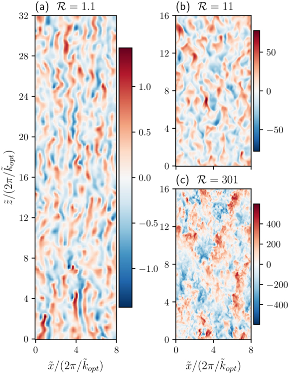
Examples of simulated thermohaline convection. These snapshots show the vertical velocity across a slice through the simulation volume. Click to enlarge. [Fraser 2026]
One of the most important parameters for modeling mixing is the Prandtl number, Pr, which is the ratio of viscosity to thermal diffusivity (in other words, a way of describing whether momentum or heat diffuses more quickly within a fluid). For stellar interiors, Pr is around 10−6, but computational limitations have prevented modelers from setting this value lower than around 10−2. When tensions between models and reality arise, this gap between simulated and realistic Pr values is often assumed to be the source of the mismatch.
Bridging the Prandtl Number Gap
In a recent research article, Adrian Fraser (University of Colorado Boulder) aimed to test this assumption. Fraser carried out 3D simulations of thermohaline mixing, using a semi-implicit modeling technique that lowered the computational cost and allowed the simulations to probe Pr values of 10−1, 10−2, 10−3, 10−6, and 0.
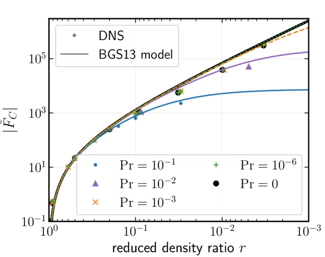
Turbulent compositional flux as a function of reduced density ratio for the simulations from this work (DNS) and the benchmark model of thermohaline convection (BGS13). Click to enlarge. [Adapted from Fraser 2026]
Recreating Reality
Where does this leave modelers attempting to recreate the reality of stellar interiors? First, a silver lining of this investigation: Fraser found that setting Pr = 0 delivered nearly identical results to Pr = 10−6. This suggests that valid results can be attained in a much less computationally intensive way, since setting Pr = 0 lowers the complexity of the simulation. While simulations with Pr = 0 may not be appropriate for all scenarios, including systems with strong magnetic fields, it may provide a way forward in certain situations.
For modeling of red giants and white dwarfs, Fraser suggested that incorporating magnetic fields, stellar rotation, or additional sources of mixing may resolve the current discrepancies. In fact, some modeling work has shown that magnetic fields could entirely close the gap between observations and models for red giant surface abundances — suggesting that bringing models and observations into agreement may be within reach.
Citation
“Bridging the Prandtl Number Gap: 3D Simulations of Thermohaline Convection in Astrophysical Regimes,” Adrian E. Fraser 2026 ApJL 1001 L22. doi:10.3847/2041-8213/ae5796