
Editor’s Note: Astrobites is a graduate-student-run organization that digests astrophysical literature for undergraduate students. As part of the partnership between the AAS and astrobites, we occasionally repost astrobites content here at AAS Nova. We hope you enjoy this post from astrobites; the original can be viewed at astrobites.org.
Title: Deconvolution of JWST/MIRI Images: Applications to an AGN Model and GATOS Observations of NGC 5728
Authors: M. T. Leist et al.
First Author’s Institution: The University of Texas at San Antonio
Status: Published in AJ
Optical Instrumentation 101
When it comes to optical instrumentation in astronomy, one of the fundamental principles is the Rayleigh criterion for angular resolution: how far apart on the sky do two sources need to be for you to distinguish them from each other? For single-piece circular apertures — i.e., most apertures smaller than about 5 meters — the angular scale is famously defined as 1.22 λ/D, where λ is the wavelength you’re observing at and D is the diameter of your aperture. This equation comes from taking the Fourier transform (a translation from spatial information to spatial frequency information) of a circular aperture and describes how the aperture “responds” to light coming in. This response is more commonly referred to as the point spread function, in part because it describes how a point source (like most stars) looks on your detector. More specifically, what your detector sees is the convolution of the point source with the point spread function. An example of this is shown in Figure 1.
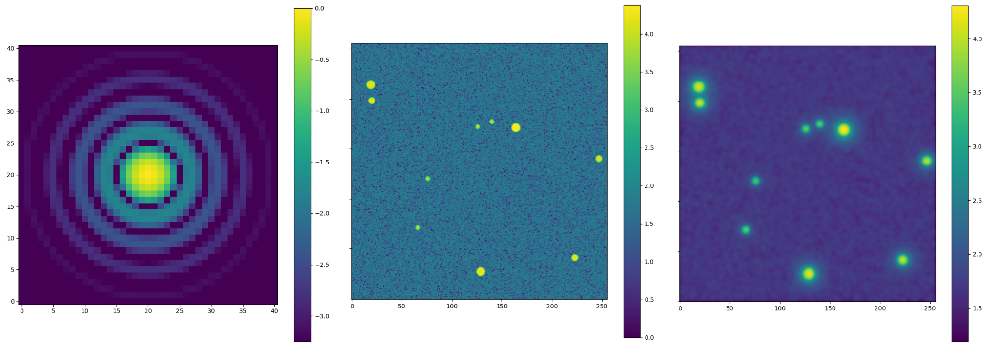
Figure 1: From left to right: 1) A point spread function for a circular aperture made from the AiryDisk2DKernel class, a part of astropy’s convolution module; 2) a fake field of stars acting as “true sources” made using the random module in numpy and the CircularAperture class in photutils; and 3) the convolution between the point spread function and the field of stars to make a model image of how a telescope might see the star field, done using the convolve function of astropy’s convolution module. This is a very simplified version of the model image building that the authors do, and you can play around with the parameters yourself here! [Ivey Davis]
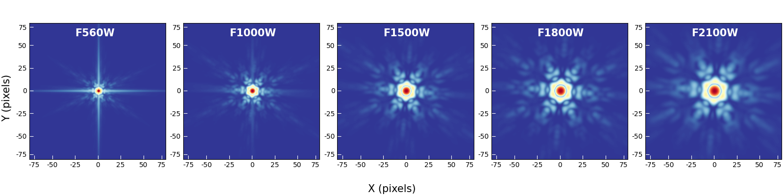
Figure 2: Modeled JWST point spread functions of five different filters ranging from 5.6 microns (leftmost panel) to 21 microns (rightmost panel) made with the WebbPSF package. [Leist et al. 2024]
This Work
To figure out how effectively they can deconvolve a JWST image of an active galactic nucleus, the authors start by building a model image of what they expect the active galactic nucleus to look like to JWST’s mid-infrared imaging instrument, MIRI. This way, they’ll know what the deconvolved image is supposed to look like and can thus better evaluate the performance of the deconvolution methods.
Their active galactic nucleus model has four components: 1) The central region of the active galactic nucleus (panel 1 in Figure 3); 2) long, collimated outflows of dust originating from the poles of the central region, called polar outflows (panel 2 in Figure 3); 3) two cones of ionization, called ionization bicones, that are commonly seen in certain types of active galactic nuclei (panel 3 in Figure 3); and 4) the host galaxy of the active galactic nucleus, taken here to be the galaxy NGC 5728 (panel 4 in Figure 3). While the host galaxy and the ionization bicones can be resolved and are thus extended features, the polar outflows can only be resolved along one axis, and the central region appears only as a point source. This makes the model a really rigorous example for the effects of both the point spread function and the deconvolution processes.
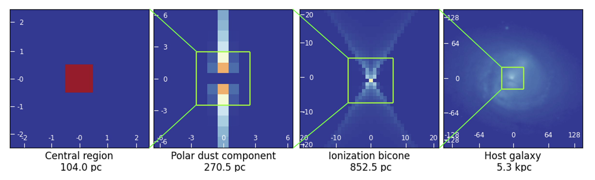
Figure 3: The four components of the active galactic nucleus model used as a “real source” for the model JWST observation. [Leist et al. 2024]
Of the five deconvolution methods used, the method that improved the point spread function the most, and did so at all wavelengths, was a method called Kraken deconvolution. Not only did it improve the point spread function the most, but it also did it in the fewest number of iterations — 22 iterations at most, while all other methods required between 29 and 105 iterations. Despite the quality of Kraken’s performance, it was not able to make the polar outflow component detectable. Regardless, the method showed true improvement in image quality and so was used to deconvolve a real JWST observation of NGC 5728 that was collected as a part of the Galactic Activity, Torus, and Outflow Survey (GATOS).
The original JWST image of NGC 5728 and the results of running the Kraken deconvolution method are shown in Figure 4. The Kraken method deconvolved the JWST image both in a similar number of iterations as well as to a similar quality as it had for the mock observation, meaning the results are consistent with expectations! The results also reveal extended structure to the south east of the central region, as shown in Figure 4. Although this feature had been observed in 2019 with other instruments, it would be undetectable in JWST images without the deconvolution technique.
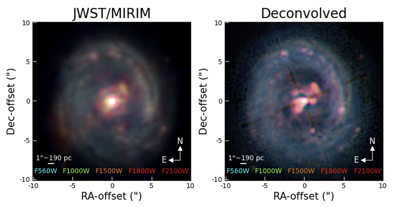
Figure 4: The JWST observation of NGC 5728 as observed by the MIRI instrument (left) and the result of deconvolving the image using the Kraken method (right). Although the outflow is indistinguishable in the original JWST image, it is readily observed to the bottom left of the central region in the deconvolved image. [Leist et al. 2024]
Original astrobite edited by Isabella Trierweiler.
About the author, Ivey Davis:
I’m a fourth-year astrophysics grad student working on the radio and optical instrumentation and science for studying magnetic activity on stars. When I’m not crying over radio-frequency interference, I’m usually baking, knitting, harassing my cat, or playing the banjo!