
Editor’s note: Astrobites is a graduate-student-run organization that digests astrophysical literature for undergraduate students. As part of the partnership between the AAS and astrobites, we occasionally repost astrobites content here at AAS Nova. We hope you enjoy this post from astrobites; the original can be viewed at astrobites.org!
Title: Fast Radio Burst 121102 Pulse Detection and Periodicity: A Machine Learning Approach
Authors: Yunfan Gerry Zhang, Vishal Gajjar, Griffin Foster, Andrew Siemion, James Cordes, Casey Law, Yu Wang
First Author’s Institution: McGill University of California Berkeley
Status: Submitted to ApJ
Today’s astrobite combines two independently fascinating topics — machine learning and fast radio bursts (FRBs) — for a very interesting result. The field of machine learning is moving at an unprecedented pace with fascinating new results. FRBs have entirely unknown origins, and experiments to detect more of them are gearing up. So let’s jump right into it and take a look at how the authors of today’s astrobite got a machine to identify fast radio bursts.
Convolutional Neural Networks
Let’s begin by introducing the technique and machinery the authors employed for finding these signals. The field of machine learning is exceptionally hot right now, and with new understanding being introduced almost daily into the best machine-learning algorithms, the diffusion into nearby fields is accelerating. This is of course no exception for astronomy (radio or otherwise), where datasets grow to be extraordinarily large and intractable for classical algorithms. Enter the Convolutional Neural Network (CNN): the go-to machine-learning algorithm for understanding and prediction on data with spatial features (aka images). How does one of these fancy algorithms work? A basic starting point would be that of a traditional neural network, but I’ll leave that explanation to someone else. A generic neural network can take in few or many inputs, but the inputs don’t necessarily have to be spatially related to each other; CNNs, however, are well suited for images. (Note: you can also have one-dimensional or three-dimensional CNNs). These images have features that, when combined, are important for identifying what is in the image. In Figure 1, for example, the dog has features such as floppy ears, or a large mouth with a tongue protruding. A CNN learns some or all of these features from a provided training dataset with a known ground truth; in Figure 1, for instance, the prediction can be labeled dog, cat, lion, or bird. These features are learned at varying spatial scales as the input images are successively convolved over, and the prediction is compared to its known label, with any corrections propagated backwards to update those features. This latter step is the training part — which you might notice is the same process as a non-convolutional neural network. Thus armed with this blazingly fast classifier, we can move forward to understanding what we’ll be predicting on.

Figure 1: An example of a convolutional neural network. An input image is sequentially convolved over through several convolutional layers, where each successive layer learns unique features, which after training, are ultimately used to make a prediction based on a set of labels. [KDnuggets]
Fast Radio Bursts
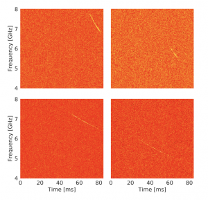
Figure 2: Simulated FRB pulses in Green Bank Telescope (GBT) radio time-frequency data. Pulses are simulated with a variety of parameters for the purpose of making the CNN as robust as possible. [Zhang et al. 2018]
Using all of these characteristics to define a training dataset, the authors simulated many different types of FRBs, all with their own unique values. This is important because having a large, robust training dataset means you’re more likely to have a neural network capable of robust predictions.
Putting the CNN to Work
We now have all the components: a convolutional neural network, a robust training dataset, and a monumental amount of Green Bank Telescope (GBT) data. The authors seek to probe archival data of the now pretty well known FRB 121102, which has a history of being a repeating FRB. This means that FRB 121102 is an amazing resource for understanding FRBs because we can take many measurements.
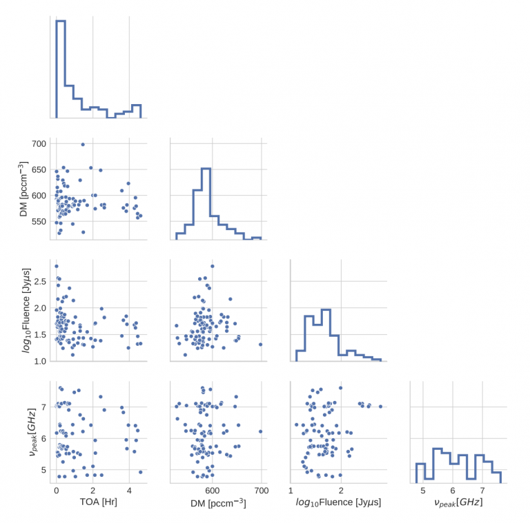
Figure 3: Distributions of the various features for the discovered FRB 121102 pulses from the GBT archival data. Understanding how these parameters relate to each other can give us hints to the nature of FRB 121102. [Zhang et al. 2018]
The additional detection and measurement of these pulses is certainly important. Like we’ve stated in our past astrobites, the origin of these bursts is almost completely speculative and we need to build up as many measurements as we can to either rule out or constrain the potential cosmological sources. Having a repeating FRB with which we can start to collect measurements, like the distributions seen in Figure 3, is fantastic for understanding the FRB’s environment affecting these parameters. Hopefully with the continued development of these CNNs and other machine-learning techniques, we’ll see an explosion of FRB detections.
About the author, Joshua Kerrigan:
I’m a 5th year PhD student at Brown University studying the early universe through the 21cm neutral hydrogen emission. I do this by using radio interferometer arrays such as the Precision Array for Probing the Epoch of Reionization (PAPER) and the Hydrogen Epoch of Reionization Array (HERA).
1 Comment
Pingback:AAS Nova – New