Preparing for the Temperature Drop at Night

Editor’s note: Astrobites is a graduate-student-run organization that digests astrophysical literature for undergraduate students. As part of the partnership between the AAS and astrobites, we repost astrobites content here at AAS Nova once a week. We hope you enjoy this post from astrobites; the original can be viewed at astrobites.org!

Title: Atmospheric circulation of hot Jupiters: dayside–nightside temperature differences
Authors: Thaddeus D. Komacek and Adam P. Showman
First Author’s Institution: University of Arizona
Status: Published in ApJ, open access

There is an old sci-fi movie “The Chronicles of Riddick” that’s set on a bizarre planet. One scene I still remember depicted the dawn on the planet. As the sun was rising (yes, somehow not tidally-locked…), the frozen surface from the night suddenly became so boiling hot that it burned anything into ash within seconds. Fortunately, on Earth, the day–night temperature difference is much milder — it’s usually less than 30°C, because the atmosphere mitigates the temperature and the Earth rotates quickly (like making evenly grilled chicken by turning it).

Hot Jupiters, on the other hand, are extreme worlds. They orbit very close to their host stars (< 0.1 AU) and are locked by the tidal force into synchronous rotation, with the same side always facing their stars. This makes for interesting atmospheric dynamics. In today’s astrobite, we take a look at these exotic worlds. The authors examined what essentially controls the day–night temperature differences and compare their theory to numerical simulations (so-called general circulation models or GCM).

The Hotter It Is, the Faster It Cools

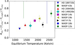
Figure 1. Normalized day–night brightness temperature difference vs. equilibrium temperature from observation of transiting hot Jupiters.

Figure 1 summarizes the observed day–night temperature difference vs. the equilibrium temperature of several most-studied hot Jupiters. The value shown on the y-axis is the normalized day–night temperature difference. The equilibrium temperature shown on the x-axis essentially tells us how close the planets are to their stars. There is clearly a trend, and the reasoning can be understood via the Stefan–Boltzmann law: the hotter (more strongly irradiated) the planet, the faster it cools (radiates). The winds cannot carry hot gas to the planet’s nightside if the heat is radiated into space too quickly. This would lead to a larger day–night temperature difference. On the other hand, if the atmospheric circulation acts efficiently enough, the winds can smear out the temperature variations by redistributing heat across the planet. Another way to look at it is that hotter planets have shorter radiative timescales. Astrophysicists like to think in terms of “timescales” while dealing with different competing processes. The process with a shorter timescale occurs faster, and it therefore dominates over the others. The authors developed a simple analytical theory that shows the dependence of day–night temperature difference, as a function of several factors: day–night equilibrium temperature difference, the timescale of radiation, and the timescale of drag. These factors, together with planetary parameters, are the key input of GCM simulation and allow a direct comparison.

Scale Analysis

Scale analysis is a powerful tool for understanding which mechanisms play important roles. The authors use scale analysis to simplify the problem and construct the theory. For example, by looking at the continuity equation, we can readily understand that  U/L ~ W/H; i.e., the ratio of the horizontal wind speed (U) to the vertical wind speed (W) is about equal to that of the planet radius (L) to the pressure scale height (H). For a typical hot Jupiter, this ratio is ~100. In other words, the observable atmosphere is thin and the horizontal flow is much faster than the vertical motion.

Pen & Paper vs. Computer

Applying scale analysis to the set of primitive equations describing the atmosphere, the authors worked out analytical expressions for various quantities, like wind speed and day–night temperature difference. Before comparing with the GCM results, let’s briefly follow their analysis based on the governing law of the gas movement — the conservation of momentum. The gas motion has four contributing factors: gas flowing in or out (advection), planet’s rotation (Coriolis force), drag force (friction), and how the pressure changes spatially (pressure gradient). The pressure gradient is the driving force of the circulation, which has to be balanced by the others. Depending on whether drag, Coriolis force, or advection dominates, the atmosphere may be in different regimes and behave differently. When rotation is important compared to advection, the pressure gradient is balanced by rotation (weak-drag) or by drag force (strong-drag), but when rotation is negligible compared to advection (slow rotation or near the equator), the pressure gradient is balanced by advection (weak-drag) or by drag force (strong-drag).

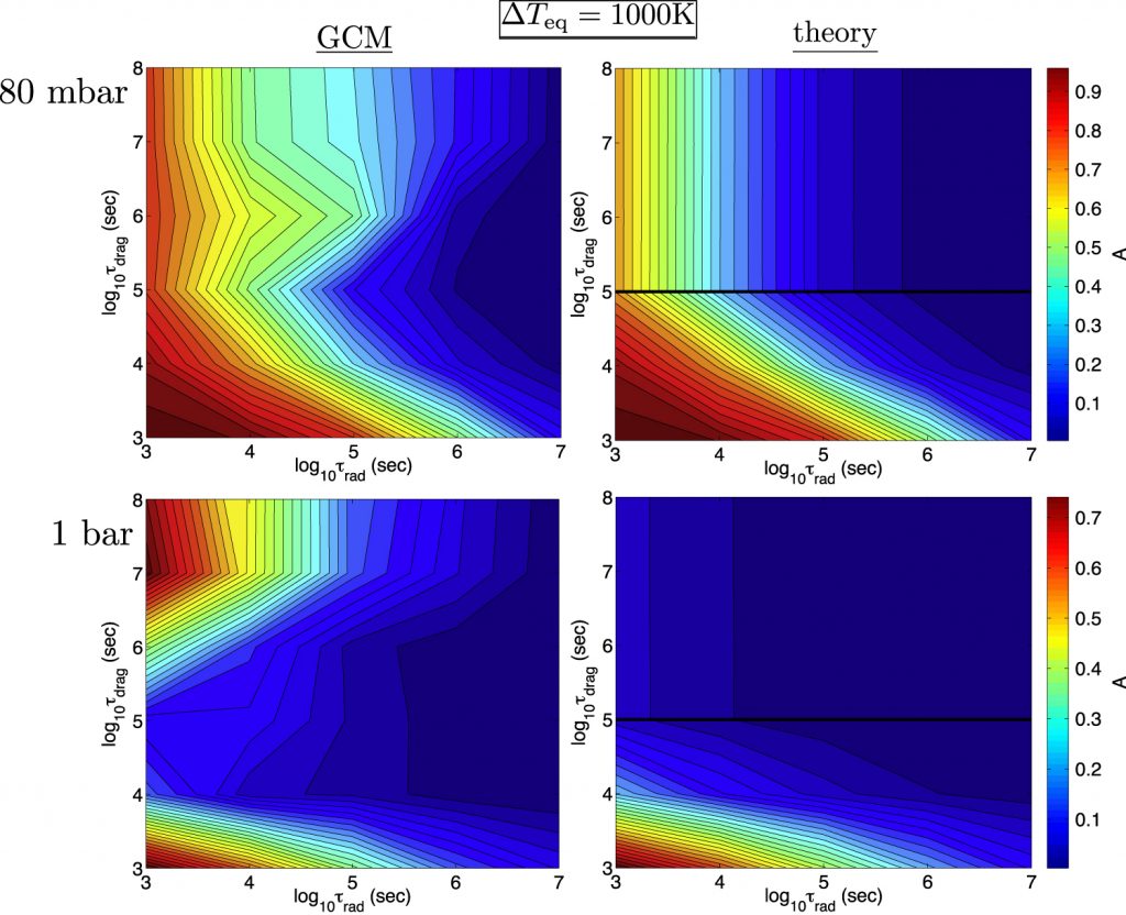
Figure 2. Overall day–night temperature difference (colors) as a function of radiative timescale and drag timescale, showing a comparison of the GCM results (left) and theory (right). The black line in the right panels indicates the transition from drag dominance to rotation dominance.

The theoretical prediction is compared to GCM results in Figure 2, showing the day–night difference for various values of drag timescales and radiative timescales for the rotation-important regime. Firstly, the day–night difference decreases as radiative timescale increases, in accordance with the trend observed. Secondly, the day–night difference has no dependence on the drag timescale until the drag timescale is shorter than ~10⁵ s (the black line in the righthand panels). This indicates the transition as discussed above: the weak-drag regime lies above the black line and the strong-drag regime under it. Lastly, a term that corresponds to the timescale of wave propagation appears in the analytical solutions in all regimes. These waves are similar to the waves in the tropics on Earth, which are strongly connected to the climate. The relative value of the wave timescale essentially controls the day–night temperature difference. It implies the wave propagation is crucial to mediate the day–night temperature difference (read more about this here).

In addition, the circulation and temperature structures in the GCM are displayed in Figure 3. Again, the radiative timescale predominantly determines the day–night temperature difference, until the drag becomes strong enough and the equatorial jet vanishes, exhibiting a symmetric circulation pattern.   

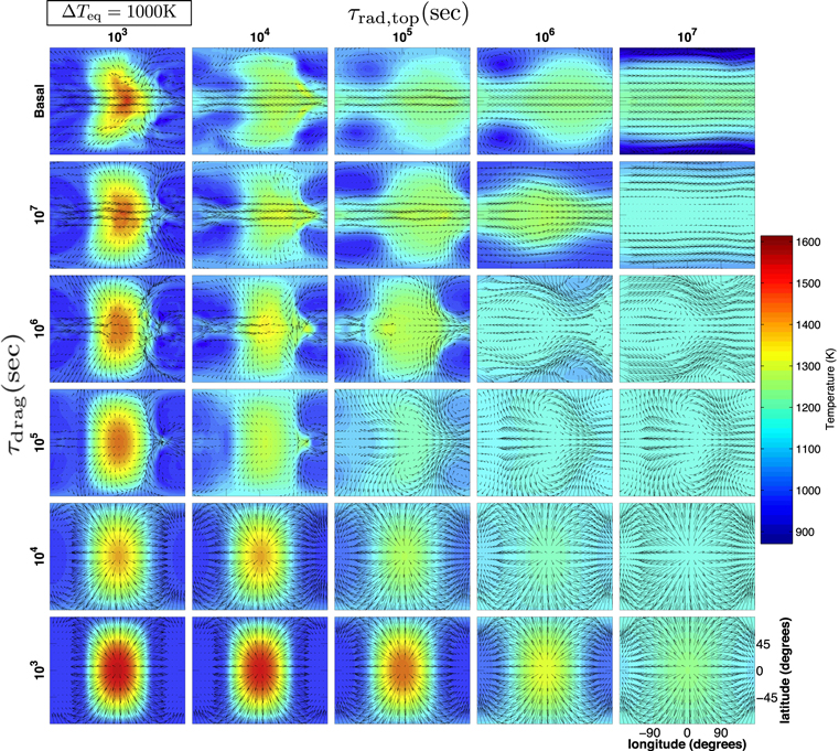
Figure 3: How temperature (colors) and wind (vectors) in GCM simulations vary with drag timescales (the y direction) and radiative timescales (the x direction).

This simple scaling theory helps us to understand the leading role of the dynamics and tells us a useful story about the physics behind it. It is always nice to see successful pen-and-paper solutions that help decipher the intricate results of computer simulations!

About the author, Shang-Min Tsai:

I am a 3rd year PhD student at the University of Bern and part of the Exoplanets & Exoclimes Group led by Prof. Kevin Heng. We are developing various open-source tools to study exoplanets. I work on modelling of atmospheric chemistry and dynamics. When I am not coding or debugging, I enjoy basketball and playing board games.